library(geomorph)
library(dplyr)
library(tidyr)
library(ggplot2)
library(effectsize)
library(ggrepel)
library(ggExtra)The following is the exact supplemental Rmarkdown file from this Journal of Archaeological Science article. It contains a bunch of extra analyses, like a consideration of intra- and interanalyst error.
INTRODUCTION
This Rmarkdown file is organized into six major sections: Introduction, Packages Needed, Validating Centroid Size-Based Body Size Reconstruction, Archaeological Body Size Estimations, Modern Comparisons, and Intra- Interindividual Error Testing. This file corresponds to analyses and figures produced in the manuscript Body Size from Unconventional Specimens. However, it also provides supplemental figures and analyses not presented in the body of the manuscript. All data are directly imported from their most raw formats (housed in corresponding folders in this Supplemental file) so that data manipulation is explicit and analyses are reproducible. The section INTRA- AND INTERINDIVIDUAL ERROR TESTING and the subsection Error Associated with SL to TL Length-Length Conversion are referenced to in the manuscript but statistical analyses and interpretation are presented here.
PACKAGES NEEDED
VALIDATING CENTROID SIZE-BASED BODY SIZE RECONSTRUCTION
mydata <-read.table(
  "Validating Centroid Size/Vertebra_Analysis_Centroid.txt", header=TRUE,
  row.names=1, stringsAsFactors = FALSE)

body.size <- read.table("Basic Files/Body_Size.txt", header=TRUE)

width <- read.table("Validating Centroid Size/Vertebra_Analysis_Width.txt",
                    header=TRUE)

species <- read.table("Basic Files/Species.txt", header=TRUE)

a <-arrayspecs(mydata, ncol(mydata)/3, 3)

mydata.gpa <- gpagen(a, curves = NULL, surfaces = NULL, PrinAxes = TRUE,
                     max.iter = NULL, ProcD = TRUE, Proj = TRUE,
                     print.progress = FALSE)

centroid.df <- data.frame(mydata.gpa$Csize)
centroid.df <- tibble::rownames_to_column(centroid.df, "ID")

centroid.clean <- centroid.df %>%
  separate("ID", into = c("ID", "Vert_Num")) %>%
  merge(body.size, by="ID") %>%
  dplyr::rename(Csize = mydata.gpa.Csize)

centroid.clean.width <- width %>%
  separate("ID", into = c("ID", "Vert_Num")) %>%
  merge(centroid.clean, by= c("ID", "Vert_Num"))

lm1 <- lm(data = centroid.clean.width, SL ~ Width)

lm2 <- lm(data = centroid.clean, SL ~ Csize)

full.dataset <- centroid.clean.width %>%
  mutate(Size.Centroid = (lm2$coefficients[[2]]*Csize)+lm2$coefficients[[1]],
         Size.Width = (lm1$coefficients[[2]]*Width)+lm1$coefficients[[1]],
         PE.Centroid = ((SL - Size.Centroid)*100)/Size.Centroid,
         PE.Width = ((SL - Size.Width)*100)/Size.Width)

MPE <- full.dataset %>%
  group_by(ID) %>%
  dplyr::summarize(MPE.Centroid = mean(PE.Centroid),
                   MPE.Width = mean(PE.Width))
Standard Length and Centrum Width
p <- ggplot(data = full.dataset, mapping = aes(x = Width, y = SL))

p + geom_point(aes(color = ID), alpha = 0.5, size = 3) +
  geom_smooth(formula = y ~ x, method = "lm", size = 1.25,
              color = "#4d4d4d") +
  theme_classic() +
  ylim(166, 500) +
  annotate("text", x = Inf, y = 166,
           label =
             "paste(italic(R^2), \" = .91 \")",
           parse = T, hjust = 1, vjust = 0, color = "#4d4d4d") +
  labs(x = "Centrum Width (mm)", y = "Standard Length (mm)") +
  theme(legend.position = "none",
        axis.line = element_line(color = "#4d4d4d", size = 1),
        axis.text.x = element_text(color = "#4d4d4d", size = 12),
        axis.text.y = element_text(color = "#4d4d4d", size = 12),
        axis.title.x = element_text(color = "#4d4d4d", size = 14,
                                    face = "bold"),
        axis.title.y = element_text(color = "#4d4d4d", size = 14,
                                    face = "bold"),
        axis.ticks.x = element_line(color = "#4d4d4d", size = 1),
        axis.ticks.y = element_line(color = "#4d4d4d", size = 1))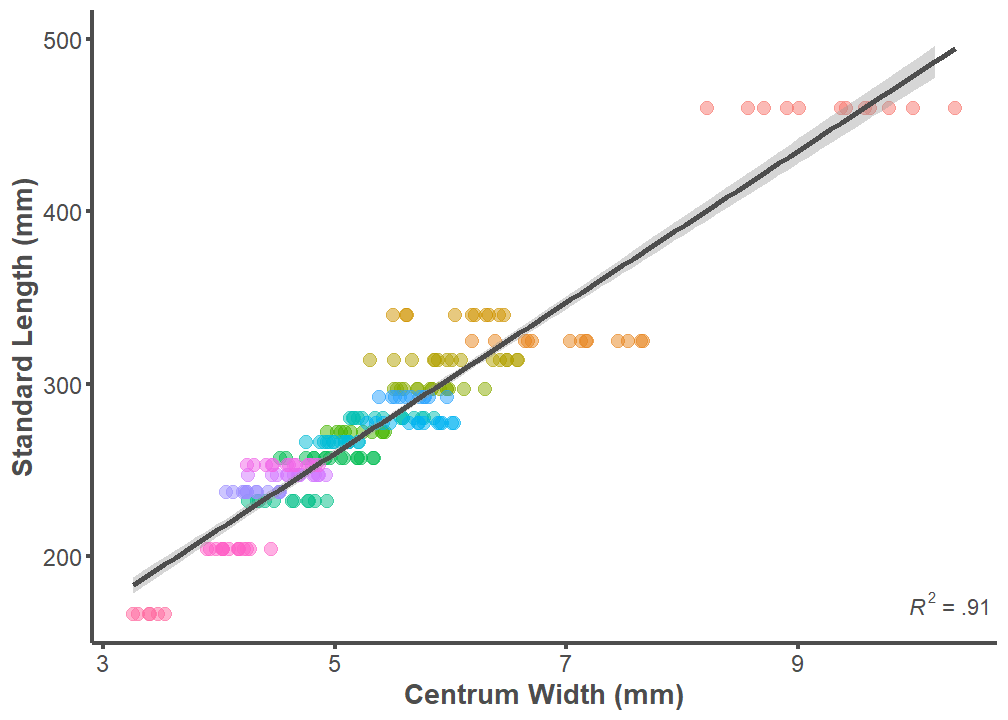
summary(lm(data = full.dataset, SL ~ Width))
Call:
lm(formula = SL ~ Width, data = full.dataset)

Residuals:
    Min      1Q  Median      3Q     Max
-51.589 -11.046   0.586  10.286  59.150

Coefficients:
            Estimate Std. Error t value Pr(>|t|)
(Intercept)  40.4340     5.3646   7.537 1.36e-12 ***
Width        43.8625     0.9596  45.711  < 2e-16 ***
---
Signif. codes:  0 '***' 0.001 '**' 0.01 '*' 0.05 '.' 0.1 ' ' 1

Residual standard error: 17.73 on 213 degrees of freedom
Multiple R-squared:  0.9075,    Adjusted R-squared:  0.9071
F-statistic:  2090 on 1 and 213 DF,  p-value: < 2.2e-16
Standard Length and Centroid Size
p <- ggplot(data = full.dataset, mapping = aes(x = Csize, y = SL))
p + geom_point(aes(color = ID), alpha = 0.5, size = 3) +
  geom_smooth(formula = y ~ x, method = "lm", size = 1.25,
              color = "#4d4d4d") +
  theme_classic() +
  ylim(166, 500) +
  annotate("text", x = Inf, y = 166,
           label =
             "paste(italic(R^2), \" = .86 \")",
           parse = T, hjust = 1, vjust = 0, color = "#4d4d4d") +
  labs(x = "Centroid Size", y = "Standard Length (mm)") +
  theme(legend.position = "none",
        axis.line = element_line(color = "#4d4d4d", size = 1),
        axis.text.x = element_text(color = "#4d4d4d", size = 12),
        axis.text.y = element_text(color = "#4d4d4d", size = 12),
        axis.title.x = element_text(color = "#4d4d4d", size = 14,
                                    face = "bold"),
        axis.title.y = element_text(color = "#4d4d4d", size = 14,
                                    face = "bold"),
        axis.ticks.x = element_line(color = "#4d4d4d", size = 1),
        axis.ticks.y = element_line(color = "#4d4d4d", size = 1))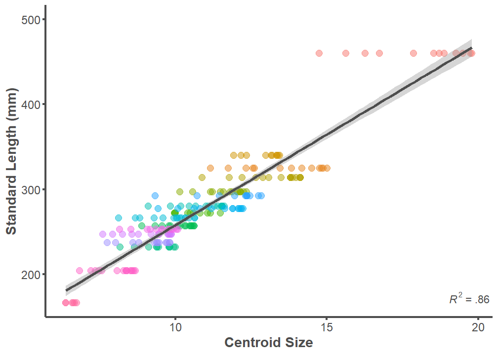
summary(lm(data = full.dataset, SL ~ Csize))
Call:
lm(formula = SL ~ Csize, data = full.dataset)

Residuals:
    Min      1Q  Median      3Q     Max
-39.810 -14.574  -3.581  12.309 100.548

Coefficients:
            Estimate Std. Error t value Pr(>|t|)
(Intercept)  44.3412     6.5309   6.789  1.1e-10 ***
Csize        21.3524     0.5783  36.920  < 2e-16 ***
---
Signif. codes:  0 '***' 0.001 '**' 0.01 '*' 0.05 '.' 0.1 ' ' 1

Residual standard error: 21.43 on 213 degrees of freedom
Multiple R-squared:  0.8649,    Adjusted R-squared:  0.8642
F-statistic:  1363 on 1 and 213 DF,  p-value: < 2.2e-16
Centrum Width Estimation and Centroid Size Estimation
p <- ggplot(data = full.dataset, mapping = aes(x = Size.Centroid,
                                                y = Size.Width))
p + geom_point(aes(color = ID), alpha = 0.5, size = 3) +
  geom_smooth(formula = y ~ x, method = "lm", size = 1.25,
              color = "#4d4d4d") +
  theme_classic() +
  annotate("text", x = Inf, y = 160,
           label = "paste(italic(R^2), \" = .94 \")",
           parse = T, hjust = 1, vjust = 0, color = "#4d4d4d") +
  labs(x = "Centroid Size Estimated Standard Length (mm)",
       y = "Centrum Width Estimated Standard Length (mm)") +
  theme(legend.position = "none",
        axis.line = element_line(color = "#4d4d4d", size = 1),
        axis.text.x = element_text(color = "#4d4d4d", size = 12),
        axis.text.y = element_text(color = "#4d4d4d", size = 12),
        axis.title.x = element_text(color = "#4d4d4d", size = 13.5,
                                    face = "bold"),
        axis.title.y = element_text(color = "#4d4d4d", size = 13.5,
                                    face = "bold"),
        axis.ticks.x = element_line(color = "#4d4d4d", size = 1),
        axis.ticks.y = element_line(color = "#4d4d4d", size = 1))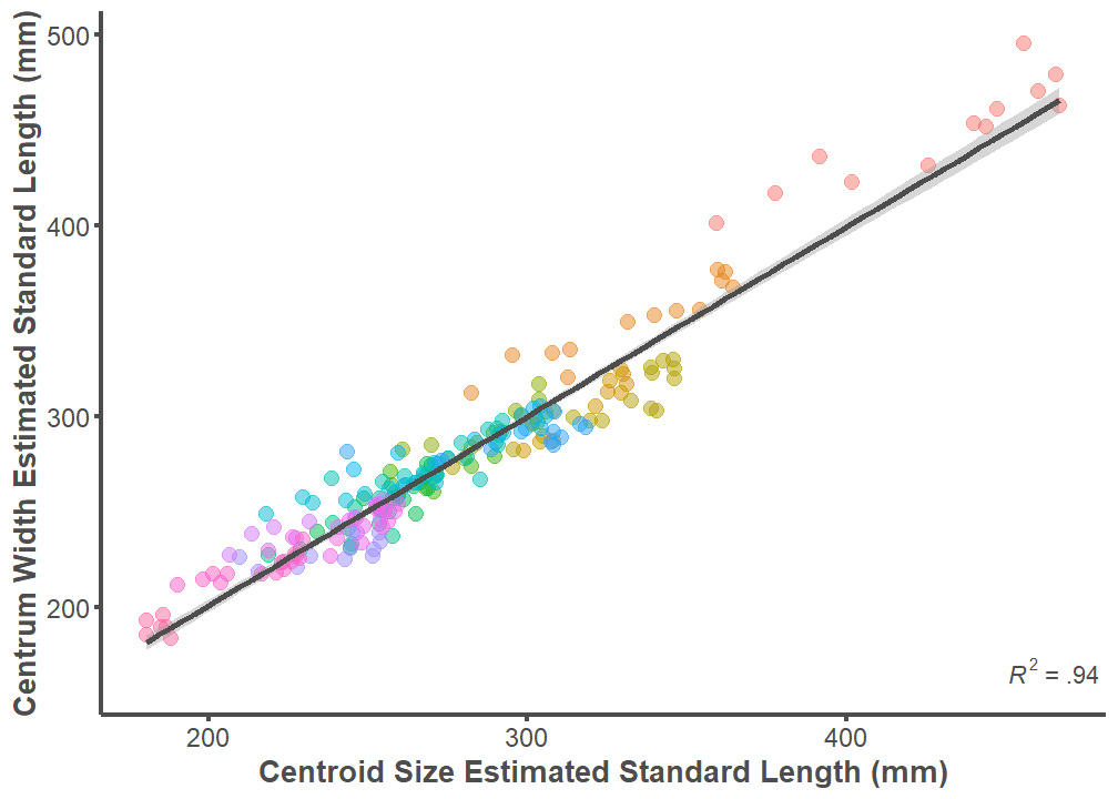
summary(lm(data = full.dataset, Size.Width ~ Size.Centroid))
Call:
lm(formula = Size.Width ~ Size.Centroid, data = full.dataset)

Residuals:
    Min      1Q  Median      3Q     Max
-37.659  -7.359  -0.599   6.340  44.890

Coefficients:
              Estimate Std. Error t value Pr(>|t|)
(Intercept)    2.42343    5.03004   0.482     0.63
Size.Centroid  0.99132    0.01768  56.072   <2e-16 ***
---
Signif. codes:  0 '***' 0.001 '**' 0.01 '*' 0.05 '.' 0.1 ' ' 1

Residual standard error: 13.99 on 213 degrees of freedom
Multiple R-squared:  0.9366,    Adjusted R-squared:  0.9363
F-statistic:  3144 on 1 and 213 DF,  p-value: < 2.2e-16
Predicion Error (PE)
p <- ggplot(data = full.dataset,
            mapping = aes(x = PE.Centroid, y = PE.Width))
p + geom_point(aes(color = ID), alpha = 0.5, size = 3) +
  geom_smooth(formula = y ~ x, method = "lm", size = 1.25,
              color = "#4d4d4d") +
  theme_classic() +
  annotate("text", x = Inf, y = -15,
           label = "paste(italic(R^2), \" = .56 \")",
           parse = T, hjust = 1, vjust = 0, color = "#4d4d4d") +
  labs(x = "PE Centroid Size", y = "PE Centrum Width") +
  theme(legend.position="none",
        axis.line = element_line(color = "#4d4d4d", size = 1),
        axis.text.x = element_text(color = "#4d4d4d", size = 12),
        axis.text.y = element_text(color = "#4d4d4d", size = 12),
        axis.title.x = element_text(color = "#4d4d4d", size = 14,
                                    face = "bold"),
        axis.title.y = element_text(color = "#4d4d4d", size = 14,
                                    face = "bold"),
        axis.ticks.x = element_line(color = "#4d4d4d", size = 1),
        axis.ticks.y = element_line(color = "#4d4d4d", size = 1))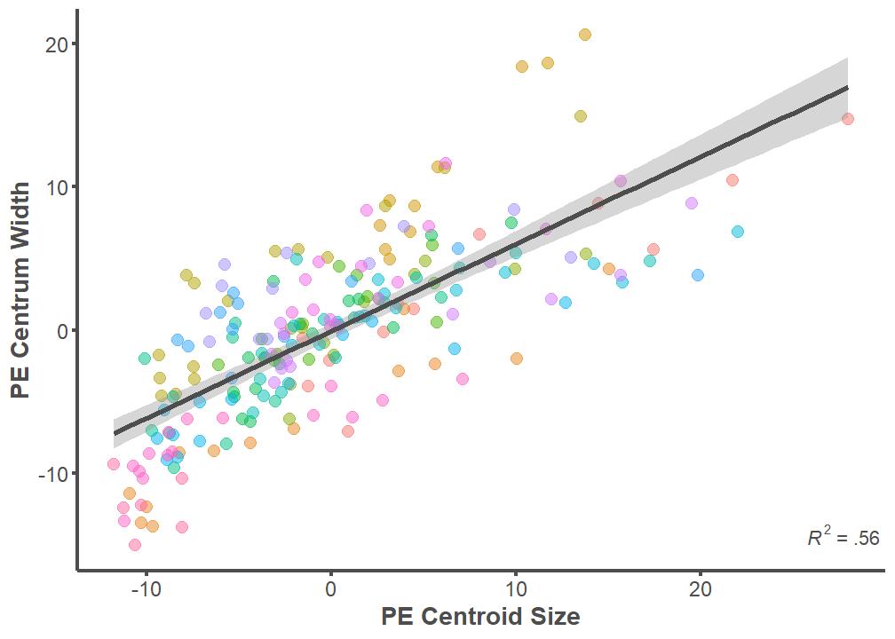
summary(lm(data = full.dataset, PE.Width ~ PE.Centroid))
Call:
lm(formula = PE.Width ~ PE.Centroid, data = full.dataset)

Residuals:
    Min      1Q  Median      3Q     Max
-8.8205 -2.8283 -0.0026  2.1242 12.3219

Coefficients:
            Estimate Std. Error t value Pr(>|t|)
(Intercept) -0.07220    0.28069  -0.257    0.797
PE.Centroid  0.60946    0.03733  16.326   <2e-16 ***
---
Signif. codes:  0 '***' 0.001 '**' 0.01 '*' 0.05 '.' 0.1 ' ' 1

Residual standard error: 4.116 on 213 degrees of freedom
Multiple R-squared:  0.5558,    Adjusted R-squared:  0.5537
F-statistic: 266.5 on 1 and 213 DF,  p-value: < 2.2e-16
Predicted SL w/ Centroid Size ~ Actual SL Centroid Size underpredits values
full.dataset %>%
  ggplot(mapping = aes(x = SL, y = Size.Centroid)) +
  geom_point(aes(color = ID), alpha = 0.5, size = 3) +
  geom_smooth(formula = y ~ x, method = "lm", size = 1.25,
              color = "#4d4d4d") +
  theme_classic() +
  labs(x = "Actual SL", y = "Predicted SL w/ Centroid Size") +
  annotate("text", x = Inf, y = 175,
           label = "paste(italic(R^2), \" = .86 \")",
           parse = T, hjust = 1, vjust = 0, color = "#4d4d4d") +
  theme(legend.position="none",
        axis.line = element_line(color = "#4d4d4d", size = 1),
        axis.text.x = element_text(color = "#4d4d4d", size = 12),
        axis.text.y = element_text(color = "#4d4d4d", size = 12),
        axis.title.x = element_text(color = "#4d4d4d", size = 14,
                                    face = "bold"),
        axis.title.y = element_text(color = "#4d4d4d", size = 14,
                                    face = "bold"),
        axis.ticks.x = element_line(color = "#4d4d4d", size = 1),
        axis.ticks.y = element_line(color = "#4d4d4d", size = 1))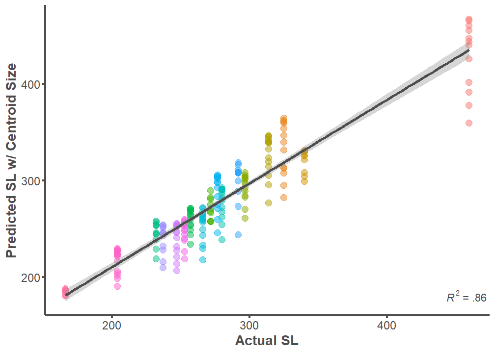
summary(lm(data = full.dataset, Size.Centroid ~ SL))
Call:
lm(formula = Size.Centroid ~ SL, data = full.dataset)

Residuals:
   Min     1Q Median     3Q    Max
-76.13 -10.50   1.93  11.25  45.98

Coefficients:
            Estimate Std. Error t value Pr(>|t|)
(Intercept) 37.75302    6.68342   5.649 5.14e-08 ***
SL           0.86485    0.02343  36.920  < 2e-16 ***
---
Signif. codes:  0 '***' 0.001 '**' 0.01 '*' 0.05 '.' 0.1 ' ' 1

Residual standard error: 19.93 on 213 degrees of freedom
Multiple R-squared:  0.8649,    Adjusted R-squared:  0.8642
F-statistic:  1363 on 1 and 213 DF,  p-value: < 2.2e-16
Predicted SL w/ Centrum Width ~ Actual SL
full.dataset %>%
  ggplot(mapping = aes(x = SL, y = Size.Width)) +
  geom_point(aes(color = ID), alpha = 0.5, size = 3) +
  geom_smooth(formula = y ~ x, method = "lm", size = 1.25,
              color = "#4d4d4d") +
  theme_classic() +
  labs(x = "Actual SL", y = "Predicted SL w/ Centrum Width") +
  annotate("text", x = Inf, y = 175,
           label = "paste(italic(R^2), \" = .91 \")",
           parse = T, hjust = 1, vjust = 0, color = "#4d4d4d") +
  theme(legend.position="none",
        axis.line = element_line(color = "#4d4d4d", size = 1),
        axis.text.x = element_text(color = "#4d4d4d", size = 12),
        axis.text.y = element_text(color = "#4d4d4d", size = 12),
        axis.title.x = element_text(color = "#4d4d4d", size = 14,
                                    face = "bold"),
        axis.title.y = element_text(color = "#4d4d4d", size = 14,
                                    face = "bold"),
        axis.ticks.x = element_line(color = "#4d4d4d", size = 1),
        axis.ticks.y = element_line(color = "#4d4d4d", size = 1))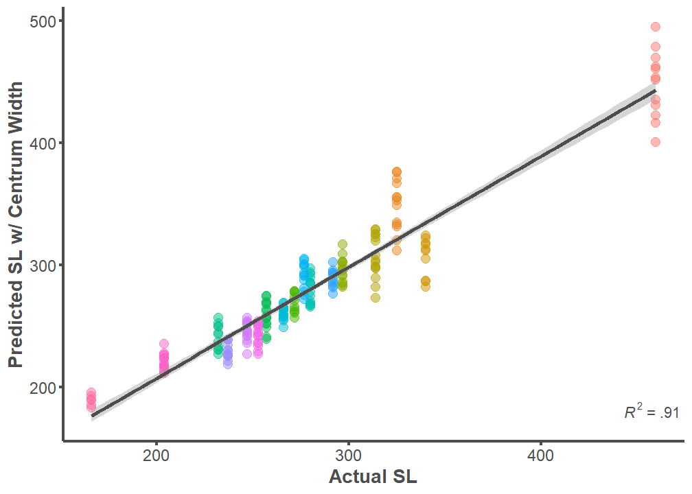
summary(lm(data = full.dataset, Size.Width ~ SL))
Call:
lm(formula = Size.Width ~ SL, data = full.dataset)

Residuals:
    Min      1Q  Median      3Q     Max
-52.495 -10.535  -1.994  10.281  55.812

Coefficients:
            Estimate Std. Error t value Pr(>|t|)
(Intercept) 25.84186    5.66415   4.562 8.54e-06 ***
SL           0.90749    0.01985  45.711  < 2e-16 ***
---
Signif. codes:  0 '***' 0.001 '**' 0.01 '*' 0.05 '.' 0.1 ' ' 1

Residual standard error: 16.89 on 213 degrees of freedom
Multiple R-squared:  0.9075,    Adjusted R-squared:  0.9071
F-statistic:  2090 on 1 and 213 DF,  p-value: < 2.2e-16
full.dataset %>%
select(PE.Centroid, PE.Width) %>%
gather(key = "PE", value = "value") %>%
ggplot(aes(x = value, color = PE, fill = PE)) +
geom_density(size = 1.5, alpha = 0.5) +
annotate(geom = "text", label = "Centroid Size", x = -5.5, y = .05, hjust = 1,
vjust = 0.5, color = "#f8766d", fontface = "bold") +
annotate(geom = "text", label = "Width", x = 4, y = .06, hjust = 0,
vjust = 0.5, color = "#00bfc4", fontface = "bold") +
theme_classic() +
theme(legend.position = "none",
axis.line = element_line(color = "#4d4d4d", size = 1),
axis.text.x = element_text(color = "#4d4d4d", size = 12),
axis.text.y = element_text(color = "#4d4d4d", size = 12),
axis.title.x = element_text(color = "#4d4d4d", size = 14,
face = "bold"),
axis.title.y = element_text(color = "#4d4d4d", size = 14,
face = "bold"),
axis.ticks.x = element_line(color = "#4d4d4d", size = 1),
axis.ticks.y = element_line(color = "#4d4d4d", size = 1)) +
geom_vline(xintercept = 0, linetype = 2, color = "#4d4d4d", size = 1) +
labs(x = "Prediction Error", y = "Density") +
scale_y_continuous(expand = c(0, 0)) +
scale_x_continuous(expand = c(0, 0))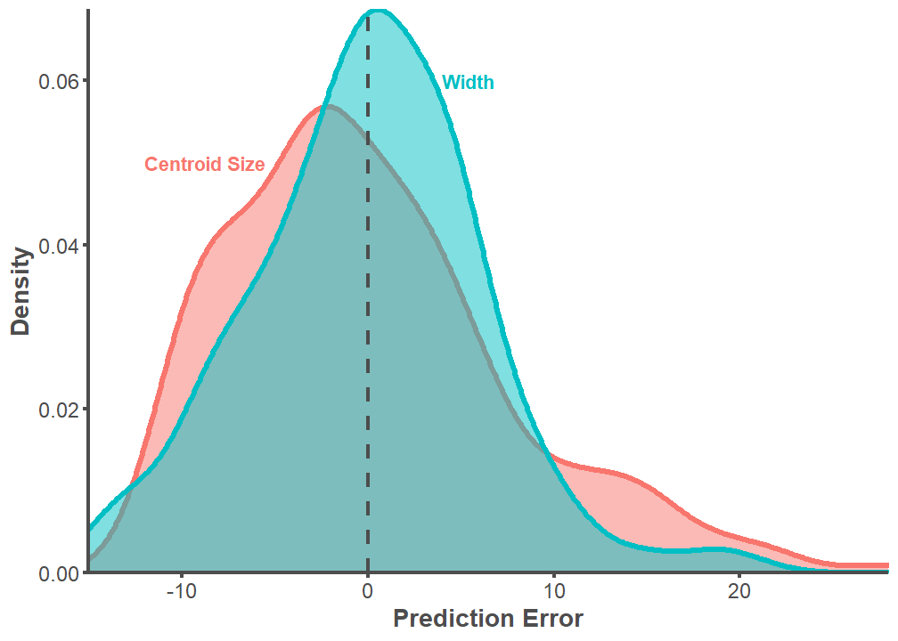
t.test(full.dataset$PE.Centroid, full.dataset$PE.Width, var.equal = TRUE)
    Two Sample t-test

data:  full.dataset$PE.Centroid and full.dataset$PE.Width
t = 0.12797, df = 428, p-value = 0.8982
alternative hypothesis: true difference in means is not equal to 0
95 percent confidence interval:
 -1.219891  1.389806
sample estimates:
  mean of x   mean of y
 0.03266882 -0.05228858
p <- ggplot(data = full.dataset,
mapping = aes(x = PE.Centroid, y = PE.Width)) +
geom_point(aes(color = ID), alpha = 0.5, size = 3) +
geom_smooth(formula = y ~ x, method = "lm", size = 1.25,
color = "#4d4d4d") +
theme_classic() +
annotate("text", x = Inf, y = -15,
label = "paste(italic(R^2), \" = .56 \")",
parse = T, hjust = 1, vjust = 0, color = "#4d4d4d") +
labs(x = "PE Centroid Size", y = "PE Centrum Width") +
theme(legend.position="none",
axis.line = element_line(color = "#4d4d4d", size = 1),
axis.text.x = element_text(color = "#4d4d4d", size = 12),
axis.text.y = element_text(color = "#4d4d4d", size = 12),
axis.title.x = element_text(color = "#4d4d4d", size = 14,
face = "bold"),
axis.title.y = element_text(color = "#4d4d4d", size = 14,
face = "bold"),
axis.ticks.x = element_line(color = "#4d4d4d", size = 1),
axis.ticks.y = element_line(color = "#4d4d4d", size = 1))
ggMarginal(p, xparams = list(color = "#f8766d", fill = "#f8766d", alpha = 0.5, size = 1.25),
yparams = list(color = "#00bfc4", fill = "#00bfc4", alpha = 0.5, size = 1.25))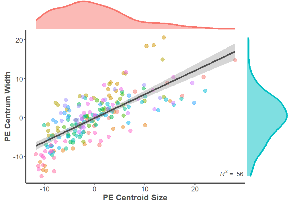
Mean Prediction Error (MPE)
p <- ggplot(data = MPE, mapping = aes(x = MPE.Centroid, y = MPE.Width))
p + geom_point(aes(color = ID), alpha = 0.5, size = 3) +
  geom_smooth(formula = y ~ x, method = "lm", size = 1.25,
              color = "#4d4d4d") +
  theme_classic() +
  annotate("text", x = Inf, y = -15,
           label = "paste(italic(R^2), \" = .63 \")",
           parse = T, hjust = 1, vjust = 0, color = "#4d4d4d") +
  labs(x = "MPE Centroid Size", y = "MPE Centrum Width") +
  theme(legend.position="none",
        axis.line = element_line(color = "#4d4d4d", size = 1),
        axis.text.x = element_text(color = "#4d4d4d", size = 12),
        axis.text.y = element_text(color = "#4d4d4d", size = 12),
        axis.title.x = element_text(color = "#4d4d4d", size = 14,
                                    face = "bold"),
        axis.title.y = element_text(color = "#4d4d4d", size = 14,
                                    face = "bold"),
        axis.ticks.x = element_line(color = "#4d4d4d", size = 1),
        axis.ticks.y = element_line(color = "#4d4d4d", size = 1))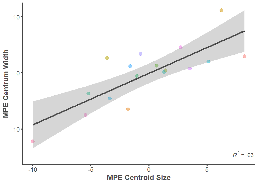
summary(lm(data = MPE, MPE.Width ~ MPE.Centroid))
Call:
lm(formula = MPE.Width ~ MPE.Centroid, data = MPE)

Residuals:
    Min      1Q  Median      3Q     Max
-4.7726 -2.4536 -0.7976  2.1232  6.0297

Coefficients:
             Estimate Std. Error t value Pr(>|t|)
(Intercept)  -0.05754    0.82072  -0.070 0.945031
MPE.Centroid  0.91819    0.18205   5.044 0.000146 ***
---
Signif. codes:  0 '***' 0.001 '**' 0.01 '*' 0.05 '.' 0.1 ' ' 1

Residual standard error: 3.38 on 15 degrees of freedom
Multiple R-squared:  0.6291,    Adjusted R-squared:  0.6043
F-statistic: 25.44 on 1 and 15 DF,  p-value: 0.0001456
ARCHAEOLOGICAL BODY SIZE ESTIMATIONS
setwd("Archaeological Estimates")
files    <- list.files(pattern = "\\.txt$")
results  <- data.frame()

for (i in seq_along(files)) {
  fname <- paste(files[i], sep="/")

  data <- read.table(fname, header = T, row.names = 1,
                     stringsAsFactors = FALSE)

  a <-arrayspecs(data, ncol(data)/3, 3)

  mydata.gpa <- gpagen(a, curves = NULL, surfaces = NULL, PrinAxes = TRUE,
                       max.iter = NULL,
       ProcD = TRUE, Proj = TRUE, print.progress = FALSE)

  centroid.df <- data.frame(mydata.gpa$Csize)
  centroid.df <- tibble::rownames_to_column(centroid.df, "ID")

  centroid.clean <- centroid.df %>%
  separate("ID", into = "ID") %>%
  merge(body.size, by="ID") %>%
  dplyr::rename(Csize = mydata.gpa.Csize)

  fit1 <- summary(lm(data = centroid.clean, SL ~ Csize))

  fit2 <- cor.test(centroid.clean$SL, centroid.clean$Csize,
                   method = "spearman")

  Arch_Size <- (fit1$coefficients[[2]]*mydata.gpa$Csize[[1]])+
    fit1$coefficients[[1]]


  results[i,1] <- fit1$coefficients[2]
  results[i,2] <- mydata.gpa$Csize[[1]]
  results[i,3] <- fit1$coefficients[1]
  results[i,4] <- fit1$r.squared
  results[i,5] <- (fit2$estimate)^2
  results[i,6] <- Arch_Size
}

rownames(results) <- sub(".txt", "", files)
colnames(results) <- c("Slope", "Csize", "Intercept", "R2", "Rho2",
                       "Arch_SL")

round(results, digits = 2)
Slope Csize Intercept R2 Rho2 Arch_SL
1304_BS 33.31 10.89 -21.54 0.90 0.89 341.36
1554_UV1 18.39 19.17 -38.22 0.81 0.61 314.26
1567_HYO 51.16 8.21 63.92 0.79 0.61 484.12
2005.27.142_HYO_UI30 51.16 5.26 63.92 0.79 0.61 332.85
2005.27.152_CV1_UI32 24.36 11.56 45.47 0.86 0.83 327.14
2005.27.152_CV2_UI32 43.17 6.60 48.47 0.87 0.85 333.31
2005.27.152_HYO_UI33 51.16 8.97 63.92 0.79 0.61 522.60
2005.27.157_UR_UI24 22.55 19.67 44.57 0.92 0.78 488.07
2005.27.158_CV_UI26 21.35 15.74 44.34 0.86 0.83 380.45
2005.27.161_UV_UI25 76.16 3.69 -1.53 0.92 0.88 279.78
2005.27.165_CV_UI29 23.17 16.89 44.46 0.87 0.84 435.78
2005.27.168_OPC_UI42 49.87 7.08 86.66 0.69 0.52 439.77
2005.27.169_CV1_U31 43.17 8.96 48.47 0.87 0.85 435.30
2005.27.169_CV2_U31 43.17 8.90 48.47 0.87 0.85 432.67
2005.27.169_CV3_U31 43.17 6.36 48.47 0.87 0.85 323.04
2005.27.169_CV4_U31 43.17 6.28 48.47 0.87 0.85 319.70
2005.27.173_CV1_U40 43.17 8.00 48.47 0.87 0.85 393.66
2005.27.173_CV2_U40 43.17 7.46 48.47 0.87 0.85 370.38
2005.27.331_CV_UI46 43.17 7.54 48.47 0.87 0.85 373.87
2005.27.331_UV_UI46 59.44 7.65 8.80 0.95 0.95 463.64
2005.27.458_CV_UI20 49.18 8.86 44.85 0.83 0.76 480.79
2007.46.1098_CV_UI3 43.17 9.73 48.47 0.87 0.85 468.56
2007.46.1100_SUB 15.11 32.93 -60.75 0.87 0.91 437.01
2007.46.2161_UI16_1 43.17 9.63 48.47 0.87 0.85 464.34
2007.46.2161_UI16_10 43.17 7.79 48.47 0.87 0.85 384.60
2007.46.2161_UI16_11 43.17 7.39 48.47 0.87 0.85 367.40
2007.46.2161_UI16_12 43.17 5.85 48.47 0.87 0.85 300.82
2007.46.2161_UI16_13 43.17 3.30 48.47 0.87 0.85 191.04
2007.46.2161_UI16_2 43.17 9.65 48.47 0.87 0.85 464.91
2007.46.2161_UI16_3 43.17 9.96 48.47 0.87 0.85 478.27
2007.46.2161_UI16_4 43.17 9.46 48.47 0.87 0.85 456.80
2007.46.2161_UI16_5 43.17 9.20 48.47 0.87 0.85 445.48
2007.46.2161_UI16_6 43.17 9.51 48.47 0.87 0.85 459.00
2007.46.2161_UI16_7 43.17 8.92 48.47 0.87 0.85 433.40
2007.46.2161_UI16_8 43.17 8.48 48.47 0.87 0.85 414.56
2007.46.2161_UI16_9 43.17 8.17 48.47 0.87 0.85 401.04
2007.46.2207_CV_UI15 43.17 10.66 48.47 0.87 0.85 508.51
2007.46.3104_BS_UI62 33.31 12.62 -21.54 0.90 0.89 398.77
2007.46.3442_CV_UI61 43.17 11.28 48.47 0.87 0.85 535.31
2007.46.4008_CT_UI53 24.24 20.57 -9.90 0.87 0.77 488.75
2007.46.4164_SUB_UI78 22.16 22.47 3.66 0.84 0.65 501.69
205.27.167_CV_UI43 52.22 9.23 48.15 0.90 0.89 530.09
205.27.167_HYO_UI43 18.17 12.57 84.31 0.70 0.46 312.58
523_MX 35.90 9.69 84.54 0.83 0.64 432.34
90.20.1199_BS_UI19 33.31 14.46 -21.54 0.90 0.89 460.17
99.20.1111_CT_UI68 26.86 8.10 74.48 0.54 0.44 291.98
99.20.1150_PT_UI58 26.88 11.55 15.55 0.99 0.98 325.84
99.20.160_UV_UI74 59.44 9.14 8.80 0.95 0.95 552.24
99.20.363_UV_UI73 18.39 21.42 -38.22 0.81 0.61 355.58
99.20.9_QUA_UI70 13.02 20.47 58.55 0.76 0.67 325.10
99.22.1765_CV_UI71 21.35 18.09 44.34 0.86 0.83 430.52
99.22.2640_OPC_UI72 49.87 8.04 86.66 0.69 0.52 487.53
99.22.3136_CV_UI8 21.35 18.37 44.34 0.86 0.83 436.54
99.22.882_OPC_UI11 49.87 7.36 86.66 0.69 0.52 453.59
BK.70.71_CT 26.86 8.11 74.48 0.54 0.44 292.29
BK.70.71_CV 43.17 6.43 48.47 0.87 0.85 326.11
BK.70.71_HYO 51.16 5.13 63.92 0.79 0.61 326.53
BK.70.71_MET 23.02 14.09 6.88 0.93 0.76 331.21
BK.70.71_UV 59.44 5.44 8.80 0.95 0.95 331.89
FN51_ENT 38.94 7.15 117.45 0.67 0.38 395.94Visualize Archaeological Distribution
results %>%
  ggplot(aes(Arch_SL)) +
  geom_density(fill = "#00bfc4", color = "#00bfc4", bw = 50, alpha = 0.5,
               size = 1.5) +
  theme_classic() +
  theme(legend.position="none",
        axis.line = element_line(color = "#4d4d4d", size = 1),
        plot.title = element_text(color = "#4d4d4d", size = 16,
                                  face = "bold"),
        axis.text.x = element_text(color = "#4d4d4d", size = 12),
        axis.text.y = element_text(color = "#4d4d4d", size = 12),
        axis.title.x = element_text(color = "#4d4d4d", size = 14,
                                    face = "bold"),
        axis.title.y = element_text(color = "#4d4d4d", size = 14,
                                    face = "bold"),
        axis.ticks.x = element_line(color = "#4d4d4d", size = 1),
        axis.ticks.y = element_line(color = "#4d4d4d", size = 1)) +
        labs(title = "Archaeological Size Distribution",
             x = "Standard Length (mm)", y = "Density") +
    xlim(0, 700)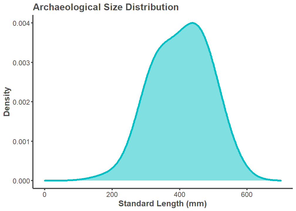
MODERN COMPARISONS
Total Length (TL)
A length-length conversion factor from Standard Length (SL) to Total Length (TL) was applied to the archaeological SL estimates. All modern comparison data uses TL. TL could not be estimated per archaeological specimen considering that two specimens from the Museum of Southwestern Biology comparative library (25273, 50002, and 50003) do not have TL measurements. A SL to TL conversion factor of 1.27 was chosen by calculating the mean values available for Ictiobus bubalus and Carpiodes carpio on fishbase.de. Available here and here.
# convert archaeological SL to TL
results <- mutate(results, Arch_TL = Arch_SL*1.27)

# visualize archaeological distribution
results %>%
  ggplot(aes(Arch_TL)) +
  geom_density(fill = "#00bfc4", color = "#00bfc4", bw = 50, alpha = 0.5,
               size = 1.5) +
  theme_classic() +
  theme(legend.position="none",
        axis.line = element_line(color = "#4d4d4d", size = 1),
        plot.title = element_text(color = "#4d4d4d", size = 16,
                                  face = "bold"),
        axis.text.x = element_text(color = "#4d4d4d", size = 12),
        axis.text.y = element_text(color = "#4d4d4d", size = 12),
        axis.title.x = element_text(color = "#4d4d4d", size = 14,
                                    face = "bold"),
        axis.title.y = element_text(color = "#4d4d4d", size = 14,
                                    face = "bold"),
        axis.ticks.x = element_line(color = "#4d4d4d", size = 1),
        axis.ticks.y = element_line(color = "#4d4d4d", size = 1)) +
        labs(title = "Archaeological Size Distribution",
             x = "Total Length (mm)", y = "Density") +
    xlim(100, 900)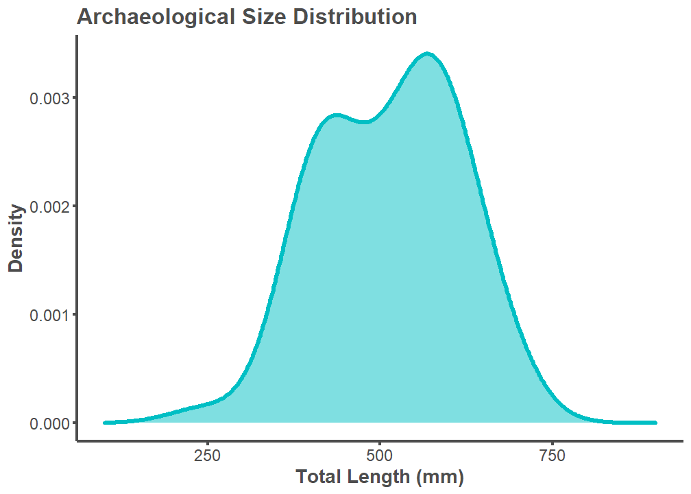
Error Associated with SL to TL Length-Length Conversion
TL and TL_estimate of specimens from the comparative library are almost perfectly correlated (R2 = 0.99; rho = 1). This means that error associated with the TL conversion factor (1.27) is extremely low. Further, the conversion factor will underestimate TL if there is error. This can be seen by visually inspecting the graph below.
body.size.estimate <- body.size %>%
  na.omit() %>%
  mutate(TL_estimate = SL * 1.27)

p <- ggplot(data = body.size.estimate,
            mapping = aes(x = TL_estimate, y = TL))
p + geom_point(alpha = 0.5, size = 4) +
  geom_smooth(formula = y ~ x, method = "lm", size = 1.25,
              color = "#4d4d4d") +
  annotate("text", x = 400, y = 215,
           label = "paste(italic(R) ^ 2, \" = .99, \", italic(rho),
           \" = 1 \")",
           parse = T, hjust = 1, vjust = 0, color = "#4d4d4d") +
  theme_classic() +
  labs(x = "Estimated Total Length (mm)", y = "Actual Total Length (mm)") +
  theme(legend.position="none",
        axis.line = element_line(color = "#4d4d4d", size = 1),
        axis.text.x = element_text(color = "#4d4d4d", size = 12),
        axis.text.y = element_text(color = "#4d4d4d", size = 12),
        axis.title.x = element_text(color = "#4d4d4d", size = 14,
                                    face = "bold"),
        axis.title.y = element_text(color = "#4d4d4d", size = 14,
                                    face = "bold"),
        axis.ticks.x = element_line(color = "#4d4d4d", size = 1),
        axis.ticks.y = element_line(color = "#4d4d4d", size = 1))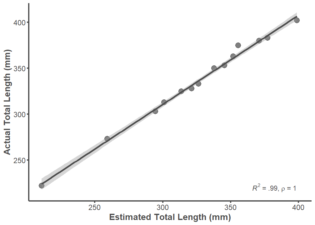
summary(lm(data = body.size.estimate, TL ~ TL_estimate))
Call:
lm(formula = TL ~ TL_estimate, data = body.size.estimate)

Residuals:
    Min      1Q  Median      3Q     Max
-4.7035 -2.6240 -0.6684  1.8637 10.3026

Coefficients:
            Estimate Std. Error t value Pr(>|t|)
(Intercept) 18.76522    7.36499   2.548   0.0256 *
TL_estimate  0.97281    0.02235  43.517 1.41e-14 ***
---
Signif. codes:  0 '***' 0.001 '**' 0.01 '*' 0.05 '.' 0.1 ' ' 1

Residual standard error: 3.968 on 12 degrees of freedom
Multiple R-squared:  0.9937,    Adjusted R-squared:  0.9932
F-statistic:  1894 on 1 and 12 DF,  p-value: 1.41e-14
rho <-cor.test(body.size.estimate$TL, body.size.estimate$TL_estimate,
method = "spearman")
rho
    Spearman's rank correlation rho

data:  body.size.estimate$TL and body.size.estimate$TL_estimate
S = 0, p-value < 2.2e-16
alternative hypothesis: true rho is not equal to 0
sample estimates:
rho
  1
Calculating Modern Comparison
Archaeological Estimates
# specify breaks
breaks <- c(-Inf,200,250,300,350,400,450,500,550,Inf)

# specify bin labels
tags <- c("-199", "200-249", "250-299", "300-349", "350-399","400-449",
          "450-499","500-549", "550+")

# put values into bins
group_tags <- cut(results$Arch_TL,
                  breaks=breaks,
                  include.lowest=TRUE,
                  right=FALSE,
                  labels=tags)

# plot
a <- as_tibble(summary(group_tags), rownames = "bins") %>%
  dplyr::rename(count = value) %>%
  mutate(percent = (count/sum(count)*100)) %>%
  dplyr::select(bins, percent) %>%
  mutate(time = "Archaeological")
Moody (1970)
# overall percentages (1967-1970) reported in Table 4
b <- tibble(bins = c("-199", "200-249", "250-299", "300-349", "350-399",
                     "400-449", "450-499","500-549", "550+"),
          percent = c(0, 2, 3, 11, 15, 21, 36, 11, 1)) %>%
  mutate(time = "Commercial")
NM Game and Fish
NMgamefish <- read.table("Modern Comparison/NM Game and Fish.txt",
                         header = TRUE)

# specify breaks
breaks <- c(-Inf, 200, 250, 300, 350, 400, 450, 500, 550, Inf)
# specify bin labels
tags <- c("-199", "200-249", "250-299", "300-349", "350-399","400-449",
          "450-499","500-549", "550+")
# puttingvalues into bins
group_tags <- cut(NMgamefish$TL,
                  breaks=breaks,
                  include.lowest=TRUE,
                  right=FALSE,
                  labels=tags)

# plot
c <- as_tibble(summary(group_tags), rownames = "bins") %>%
  dplyr::rename(count = value) %>%
  mutate(percent = (count/sum(count)*100)) %>%
  dplyr::select(bins, percent) %>%
  mutate(time = "Non_Commercial")
Bind Together and Plot
d <- rbind(a, b, c)

d$time <- factor(d$time, levels = c("Commercial", "Non_Commercial",
                                    "Archaeological"))

d$time2 <- factor(d$time,
                  labels = c("Commercial Fishery (1967–1970)",
                             "Non-Commercial Fishery (2011–2017)",
                             "Archaeological Fishery (ca. AD 1300-1600)"))

ggplot(d, aes(x = bins, y = percent)) +
  geom_bar(stat = "identity", size = 1.5) +
  facet_wrap(~ time2, nrow = 3) +
  scale_y_continuous(breaks = seq(0, 45, by = 15)) +
  theme_classic() +
  theme(legend.position="top",
        strip.text.x = element_text(color = "#4d4d4d", size = 12,
                                    face = "bold"),
        strip.background = element_rect(color= NA, fill= NA),
        legend.title = element_blank(),
        axis.line = element_line(color = "#4d4d4d", size = 1),
        axis.text.x = element_text(color = "#4d4d4d", size = 7),
        axis.text.y = element_text(color = "#4d4d4d", size = 8),
        axis.title.x = element_text(color = "#4d4d4d", size = 10,
                                    face = "bold"),
        axis.title.y = element_text(color = "#4d4d4d", size = 10,
                                    face = "bold"),
        axis.ticks.x = element_line(color = "#4d4d4d", size = 1),
        axis.ticks.y = element_line(color = "#4d4d4d", size = 1)) +
        labs(x = "Total Length (mm)", y = "Percent (%)")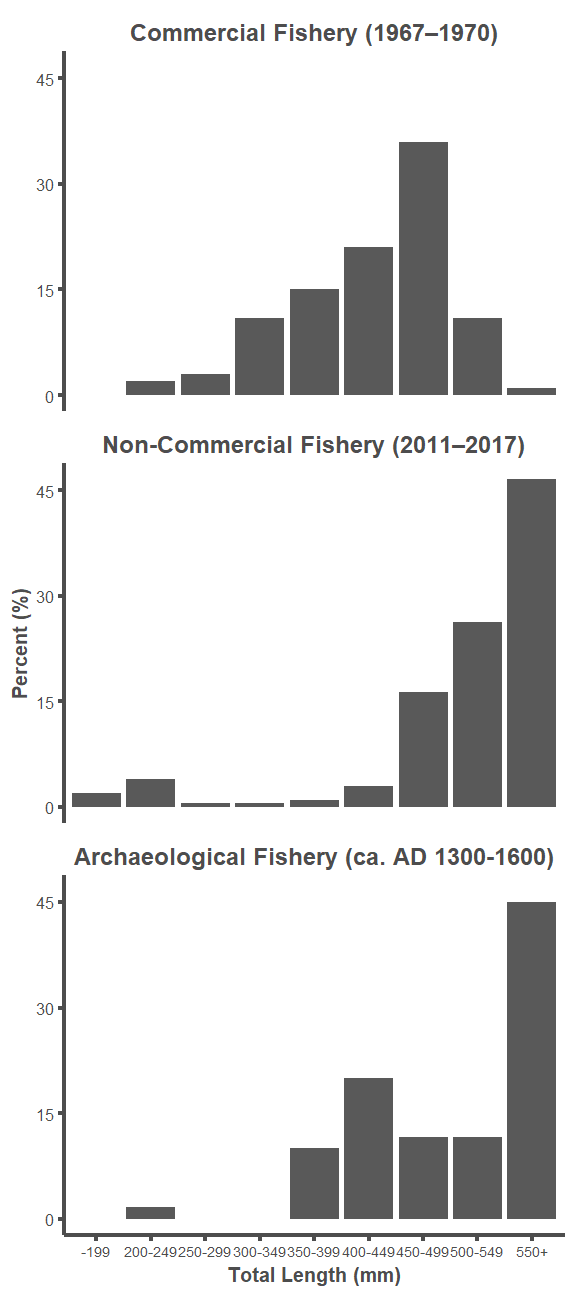
INTRA- AND INTERINDIVIDUAL ERROR TESTING
Intraobserver Error
Analyst 1 (Alexandra Harris)
Run a Generalized Procrustes Analysis for all Analyst 1 datafiles. Each .txt file pertains to a specimen and contains five replicate landmark configurations
setwd("Error Testing/Alex")
files    <- list.files(pattern = "\\.txt$")
my.list <- list()

for (i in seq_along(files)) {
  fname <- paste(files[i], sep="/")

  data <- read.table(fname, header = T, row.names = 1,
                     stringsAsFactors = FALSE)

  a <-arrayspecs(data, ncol(data)/3, 3)

  mydata.gpa <- gpagen(a, curves = NULL, surfaces = NULL, PrinAxes = TRUE,
                       max.iter = NULL,
       ProcD = TRUE, Proj = TRUE, print.progress = FALSE)

my.list[[i]] <- mydata.gpa
}
Establish number of rows in each landmark configuration
rows <- rep(NA, 60)
for(i in seq_along(my.list)){
  rows[i] <- dim(my.list[[i]][["coords"]])[1]
}
Create lists out of all coordinates per replicate per specimen and all consensuses per specimen
# initiate
coords <- list()
for(i in 1:60){
  coords[[i]] <- array(NA, dim = c(rows[i], 3, 5))
}

# isolate coordinates per specimen per analyst per replicate
for(i in seq_along(my.list)){
  for(j in 1:5){
  coords[[i]][,,j] <- my.list[[i]][["coords"]][,,j]
  }
}

# initiate
consensus <- list()

# isolate consensus per specimen
for(i in seq_along(my.list)){
  consensus[[i]] <- my.list[[c(i, 4)]]
}
Calculate procd (procd = total Procrustes distance from consensus)
# initiate
output1 <- list()
for(i in 1:60){
  output1[[i]] <- array(NA, dim = c(rows[i], 3, 5))
}

# subtract and square
for(i in seq_along(coords)){
  for(j in 1:5){
    output1[[i]][,,j] <- (coords[[i]][,,j] - consensus[[i]])^2
  }
}

# initiate
output2 <- list()
for(i in 1:60){
  output2[[i]] <- array(NA, dim = c(1, rows[i], 5))
}

# sum rows
for(i in seq_along(output1)){
  for(j in 1:5){
    output2[[i]][,,j] <- rowSums(output1[[i]][,,j])
  }
}

# initiate
procd <- list()
for(i in 1:60){
  procd[[i]] <- array(NA, dim = c(1, 1, 5))
}

# sum and square root
for(i in 1:60){
  for(j in 1:5){
    procd[[i]][,,j] <- sqrt(sum(output2[[i]][,,j]))
  }
}
Transform procd and assign to Analyst 1
# create dataframe
procd <- data.frame(unlist(procd))

#subset data for Analyst 1 and transform
analyst1.procd <- procd %>%
  mutate(analyst = "Analyst 1",
         replicate = rep(c("1", "2", "3", "4", "5"), times = 60)) %>%
  rename(procd = colnames(procd)[1])
Analyst 2 (Jonathan Dombrosky)
Run a Generalized Procrustes Analysis for all Analyst 2 datafiles. Each .txt file pertains to a specimen and contains five replicate landmark configurations
setwd("Error Testing/Jon")
files    <- list.files(pattern = "\\.txt$")
my.list <- list()

for (i in seq_along(files)) {
  fname <- paste(files[i], sep="/")

  data <- read.table(fname, header = T, row.names = 1,
                     stringsAsFactors = FALSE)

  a <-arrayspecs(data, ncol(data)/3, 3)

  mydata.gpa <- gpagen(a, curves = NULL, surfaces = NULL, PrinAxes = TRUE,
                       max.iter = NULL,
       ProcD = TRUE, Proj = TRUE, print.progress = FALSE)

my.list[[i]] <- mydata.gpa
}
Establish number of rows in each landmark configuration
rows <- rep(NA, 60)
for(i in seq_along(my.list)){
  rows[i] <- dim(my.list[[i]][["coords"]])[1]
}
Create lists out of all coordinates per replicate per specimen and all consensuses per specimen
# initiate
coords <- list()
for(i in 1:60){
  coords[[i]] <- array(NA, dim = c(rows[i], 3, 5))
}

# isolate coordinates per specimen per analyst per replicate
for(i in seq_along(my.list)){
  for(j in 1:5){
  coords[[i]][,,j] <- my.list[[i]][["coords"]][,,j]
  }
}

# initiate
consensus <- list()

# isolate consensus per specimen
for(i in seq_along(my.list)){
  consensus[[i]] <- my.list[[c(i, 4)]]
}
Calculate procd (procd = total Procrustes distance from consensus)
# initiate
output1 <- list()
for(i in 1:60){
  output1[[i]] <- array(NA, dim = c(rows[i], 3, 5))
}

# subtract and square
for(i in seq_along(coords)){
  for(j in 1:5){
    output1[[i]][,,j] <- (coords[[i]][,,j] - consensus[[i]])^2
  }
}

# initiate
output2 <- list()
for(i in 1:60){
  output2[[i]] <- array(NA, dim = c(1, rows[i], 5))
}

# sum rows
for(i in seq_along(output1)){
  for(j in 1:5){
    output2[[i]][,,j] <- rowSums(output1[[i]][,,j])
  }
}

# initiate
procd <- list()
for(i in 1:60){
  procd[[i]] <- array(NA, dim = c(1, 1, 5))
}

# sum and square root
for(i in 1:60){
  for(j in 1:5){
    procd[[i]][,,j] <- sqrt(sum(output2[[i]][,,j]))
  }
}
Transform procd and assign to Analyst 2
# create dataframe
procd <- data.frame(unlist(procd))

#subset data for Analyst 1 and transform
analyst2.procd <- procd %>%
  mutate(analyst = "Analyst 2",
         replicate = rep(c("1", "2", "3", "4", "5"), times = 60)) %>%
  rename(procd = colnames(procd)[1])
Bind Analyst 1 and Analyst 2 datasets
procd <- rbind(analyst1.procd, analyst2.procd)Visualize and Significance Testing
One way ANOVA tests indicate that the mean values of procd are equal between replicates for Analyst 1 (p = 0.91) and Analyst 2 (p = 0.31). Further, the effect size between replicates is extremely small for Analyst 1 (Eta2 < 0.01) and Analyst 2 (Eta2 = 0.02). The landmarking configurations on the entire archaeological dataset are practically indistinguishable between replicates of the same analyst.
procd %>%
  ggplot(mapping = aes(x = replicate, y = procd, group = replicate,
                       fill = replicate, color = replicate)) +
  geom_boxplot(size = 0.75, alpha = 0.5, outlier.alpha = 0.5,
               outlier.size = 2.5) +
  facet_wrap(~ analyst, nrow = 2) +
  theme_classic() +
  theme(legend.position= "none",
        strip.background = element_blank(),
        strip.text.x = element_text(color = "#4d4d4d", size = 16,
                                    face = "bold"),
        axis.line = element_line(color = "#4d4d4d", size = 1),
        axis.text.x = element_text(color = "#4d4d4d", size = 12),
        axis.text.y = element_text(color = "#4d4d4d", size = 12),
        axis.title.x = element_text(color = "#4d4d4d", size = 14,
                                    face = "bold"),
        axis.title.y = element_text(color = "#4d4d4d", size = 14,
                                    face = "bold"),
        axis.ticks.x = element_line(color = "#4d4d4d", size = 1),
        axis.ticks.y = element_line(color = "#4d4d4d", size = 1)) +
        labs(x = "Replicate", y = "Total Procrustes Distance\nfrom Consensus")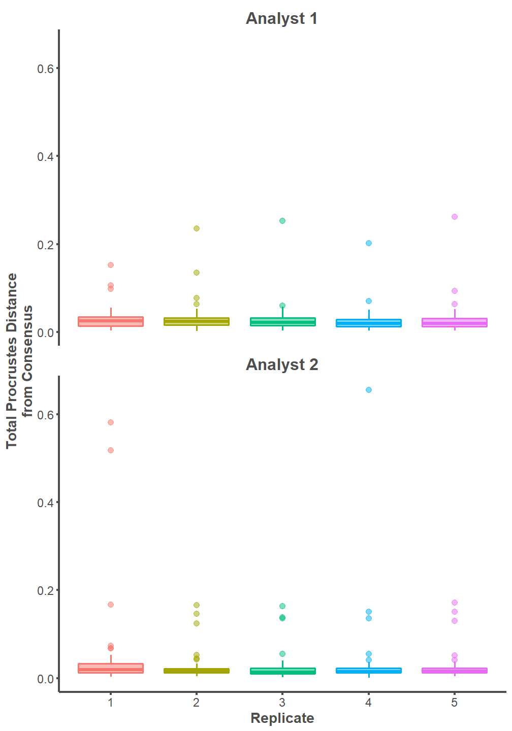
oneway.analyst1 <- aov(procd ~ replicate, data = analyst1.procd)
summary(oneway.analyst1)
Df Sum Sq Mean Sq F value Pr(>F)
replicate 4 0.00096 0.0002397 0.254 0.907
Residuals 295 0.27886 0.0009453 eta_squared(oneway.analyst1)For one-way between subjects designs, partial eta squared is equivalent
to eta squared. Returning eta squared.# Effect Size for ANOVA
Parameter | Eta2 | 95% CI
-----------------------------------
replicate | 3.43e-03 | [0.00, 1.00]
- One-sided CIs: upper bound fixed at [1.00].oneway.analyst2 <- aov(procd ~ replicate, data = analyst2.procd)
summary(oneway.analyst2) Df Sum Sq Mean Sq F value Pr(>F)
replicate 4 0.0188 0.004707 1.193 0.314
Residuals 295 1.1636 0.003944 eta_squared(oneway.analyst2)For one-way between subjects designs, partial eta squared is equivalent
to eta squared. Returning eta squared.# Effect Size for ANOVA
Parameter | Eta2 | 95% CI
-------------------------------
replicate | 0.02 | [0.00, 1.00]
- One-sided CIs: upper bound fixed at [1.00].Swarmplot
library(ggbeeswarm)

procd %>%
  ggplot(mapping = aes(x = replicate, y = procd, group = replicate,
                       fill = replicate, color = replicate)) +
  geom_beeswarm(size = 4, cex = 0.8, alpha = 0.2) +
  geom_beeswarm(size = 4, cex = 0.8, shape = 21, fill = NA) +
  facet_wrap(~ analyst, nrow = 2) +
  theme_classic() +
  theme(legend.position= "none",
        strip.background = element_blank(),
        strip.text.x = element_text(color = "#4d4d4d", size = 16,
                                    face = "bold"),
        axis.line = element_line(color = "#4d4d4d", size = 1),
        axis.text.x = element_text(color = "#4d4d4d", size = 12),
        axis.text.y = element_text(color = "#4d4d4d", size = 12),
        axis.title.x = element_text(color = "#4d4d4d", size = 14,
                                    face = "bold"),
        axis.title.y = element_text(color = "#4d4d4d", size = 14,
                                    face = "bold"),
        axis.ticks.x = element_line(color = "#4d4d4d", size = 1),
        axis.ticks.y = element_line(color = "#4d4d4d", size = 1)) +
        labs(x = "Replicate", y = "Total Procrustes Distance from Consensus")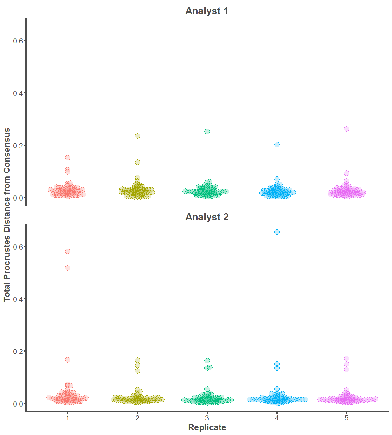
Interobserver Error
Run a Generalized Procrustes Analysis for all datafiles (both Analyst 1 and Analyst 2 combined). Each .txt file pertains to a specimen and contains five replicate landmark configurations per analyst.
setwd("Error Testing/Both")
files    <- list.files(pattern = "\\.txt$")
my.list <- list()

for (i in seq_along(files)) {
  fname <- paste(files[i], sep="/")

  data <- read.table(fname, header = T, row.names = 1,
                     stringsAsFactors = FALSE)

  a <-arrayspecs(data, ncol(data)/3, 3)

  mydata.gpa <- gpagen(a, curves = NULL, surfaces = NULL, PrinAxes = TRUE,
                       max.iter = NULL,
       ProcD = TRUE, Proj = TRUE, print.progress = FALSE)

my.list[[i]] <- mydata.gpa
}
Establish number of rows in each landmark configuration
rows <- rep(NA, 60)
for(i in seq_along(my.list)){
  rows[i] <- dim(my.list[[i]][["coords"]])[1]
}
Create lists out of all coordinates per replicate per analyst per specimen and all consensuses per specimen
# initiate
coords <- list()
for(i in 1:60){
  coords[[i]] <- array(NA, dim = c(rows[i], 3, 10))
}

# isolate coordinates per specimen per analyst per replicate
for(i in seq_along(my.list)){
  for(j in 1:10){
  coords[[i]][,,j] <- my.list[[i]][["coords"]][,,j]
  }
}

# initiate
consensus <- list()

# isolate consensus per specimen
for(i in seq_along(my.list)){
  consensus[[i]] <- my.list[[c(i, 4)]]
}
Calculate procd (procd = total Procrustes distance from consensus)
# initiate
output1 <- list()
for(i in 1:60){
  output1[[i]] <- array(NA, dim = c(rows[i], 3, 10))
}

# subtract and square
for(i in seq_along(coords)){
  for(j in 1:10){
    output1[[i]][,,j] <- (coords[[i]][,,j] - consensus[[i]])^2
  }
}

# initiate
output2 <- list()
for(i in 1:60){
  output2[[i]] <- array(NA, dim = c(1, rows[i], 10))
}

# sum rows
for(i in seq_along(output1)){
  for(j in 1:10){
    output2[[i]][,,j] <- rowSums(output1[[i]][,,j])
  }
}

# initiate
procd <- list()
for(i in 1:60){
  procd[[i]] <- array(NA, dim = c(1, 1, 10))
}

# sum and square root
for(i in 1:60){
  for(j in 1:10){
    procd[[i]][,,j] <- sqrt(sum(output2[[i]][,,j]))
  }
}
Transform procd
# create dataframe
procd <- data.frame(unlist(procd))

#subset data for Analyst 1 and transform
analyst1.procd <- data.frame(procd[c(rep(TRUE, 5), rep(FALSE, 5)),])

analyst1.procd <- analyst1.procd %>%
  mutate(analyst = "1") %>%
  rename(procd = colnames(analyst1.procd)[1])

#subset data for Analyst 2 and transform
analyst2.procd <- data.frame(procd[c(rep(FALSE, 5), rep(TRUE, 5)),])

analyst2.procd <- analyst2.procd %>%
  mutate(analyst = "2") %>%
  rename(procd = colnames(analyst2.procd)[1])

#bind transformed datasets for Analyst 1 and 2
procd <- rbind(analyst1.procd, analyst2.procd)
Visualize and Significance Testing
An independent t-test indicates that the mean values of procd between Analyst 1 and Analyst 2 are equal (p = 0.89). Further, the effect size between the two means is extremely small (Cohen’s d = 0.01). The landmarking configuration on the entire archaeological dataset (replicated five times) is practically indistinguishable between Analyst 1 and Analyst 2.
procd %>%
  ggplot(mapping = aes(x = analyst, y = procd, group = analyst,
                       fill = analyst, color = analyst)) +
  geom_boxplot(size = 0.75, alpha = 0.5, outlier.alpha = 0.5,
               outlier.size = 2.5) +
  theme_classic() +
  theme(legend.position= "none",
        strip.background = element_blank(),
        strip.text.x = element_text(color = "#4d4d4d", size = 16,
                                    face = "bold"),
        axis.line = element_line(color = "#4d4d4d", size = 1),
        axis.text.x = element_text(color = "#4d4d4d", size = 12),
        axis.text.y = element_text(color = "#4d4d4d", size = 12),
        axis.title.x = element_text(color = "#4d4d4d", size = 14,
                                    face = "bold"),
        axis.title.y = element_text(color = "#4d4d4d", size = 14,
                                    face = "bold"),
        axis.ticks.x = element_line(color = "#4d4d4d", size = 1),
        axis.ticks.y = element_line(color = "#4d4d4d", size = 1)) +
        labs(x = "Analyst", y = "Total Procrustes Distance\n from Consensus")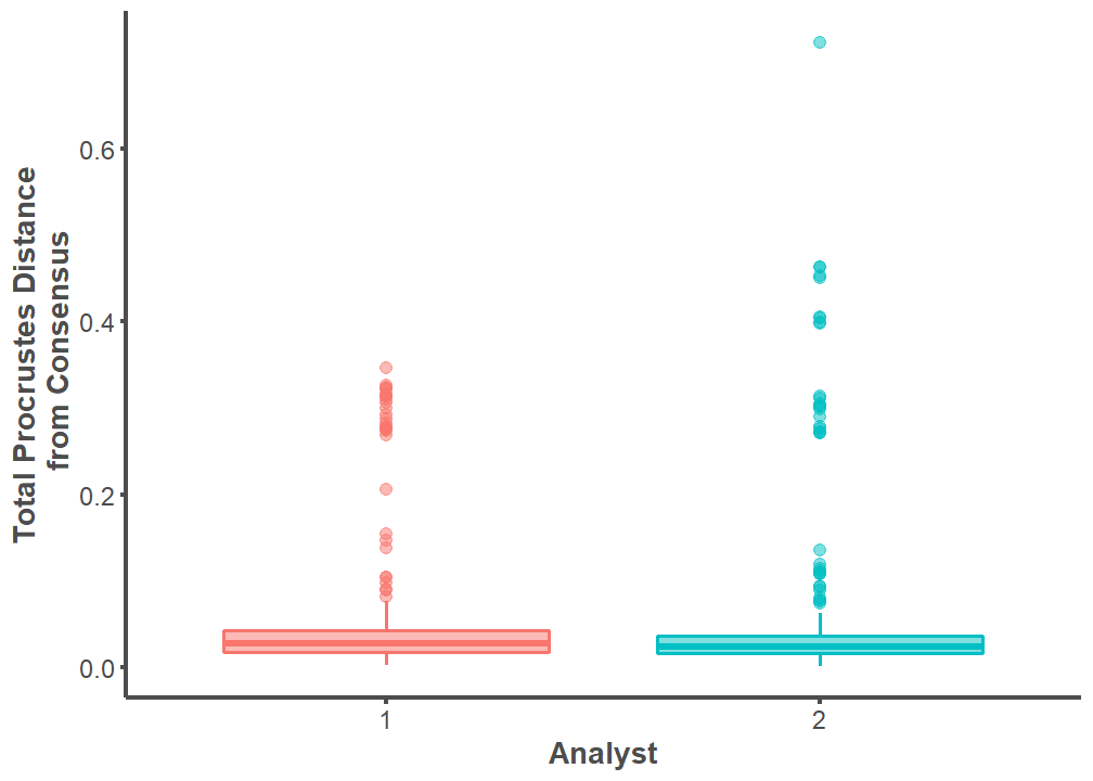
t.test <- t.test(analyst1.procd$procd, analyst2.procd$procd)
t.test
    Welch Two Sample t-test

data:  analyst1.procd$procd and analyst2.procd$procd
t = -0.13727, df = 570.74, p-value = 0.8909
alternative hypothesis: true difference in means is not equal to 0
95 percent confidence interval:
 -0.01440174  0.01252025
sample estimates:
 mean of x  mean of y
0.05045055 0.05139130 cohens_d(t.test)Cohen's d | 95% CI
-------------------------
-0.01 | [-0.17, 0.15]
- Estimated using un-pooled SD.Swarmplot
procd %>%
  ggplot(mapping = aes(x = analyst, y = procd, group = analyst,
                       fill = analyst, color = analyst)) +
  geom_beeswarm(size = 4, cex = 0.8, alpha = 0.2) +
  geom_beeswarm(size = 4, cex = 0.8, shape = 21, fill = NA) +
  theme_classic() +
  theme(legend.position= "none",
        strip.background = element_blank(),
        strip.text.x = element_text(color = "#4d4d4d", size = 16,
                                    face = "bold"),
        axis.line = element_line(color = "#4d4d4d", size = 1),
        axis.text.x = element_text(color = "#4d4d4d", size = 12),
        axis.text.y = element_text(color = "#4d4d4d", size = 12),
        axis.title.x = element_text(color = "#4d4d4d", size = 14,
                                    face = "bold"),
        axis.title.y = element_text(color = "#4d4d4d", size = 14,
                                    face = "bold"),
        axis.ticks.x = element_line(color = "#4d4d4d", size = 1),
        axis.ticks.y = element_line(color = "#4d4d4d", size = 1)) +
        labs(x = "Analyst", y = "Total Procrustes Distance\n from Consensus")