library(SIBER)
library(tidyverse)
library(cowplot)
library(broom)
library(gt)
library(ggtext)

# For the map
library(tmap)
library(sf)
library(spData)
library(spDataLarge) #https://github.com/Nowosad/spDataLarge
library(raster)
library(terra)
library(grid)The following is the supplemental material from this Journal of Archaeological Science: Reports article.
1 Libraries
2 Figure 1
2.1 Load in DEM
Link to USGS DEM. This file is required to make Figure 1, but it is not included in the GitHub repo because it is too large. Go to the link, download the file, and save it in your working directory
west_dem <- rast("dem90_hf.tif")2.2 Set Region Bounding Box
four_corners <- us_states %>%
  filter(NAME %in% c("Colorado", "New Mexico", "Arizona", "Utah"))

four_corners <-  st_transform(four_corners, crs(west_dem))

region <- st_bbox(c(xmin = -1200000, xmax = -750000, ymin = 1200000,
                    ymax = 1800000), crs = st_crs(four_corners)) %>%
  st_as_sfc()
2.3 Crop and Mask DEM with Region Bounding Box
dem_crop <- crop(west_dem, vect(region))
dem_mask <- mask(dem_crop, vect(region))
2.4 Map DEM
rast <- tm_shape(dem_mask, bbox = region) +
  tm_raster(style = "cont", palette = "Greys", legend.show = TRUE,
            title = "elevation (m)") +
  tm_scale_bar(position = c("left", "bottom"), width = .2) +
  tm_compass(type = "arrow", position = c("left", 0.09)) +
  tm_layout(legend.frame = TRUE,
            legend.outside.position = "right",
            legend.position = c("center", "bottom"),
            legend.title.size = 0.6,
            legend.text.size = 0.5,
            legend.title.fontface = "bold",
            inner.margins = c(0, 0, 0, 0))
2.5 Create Sites and Cities Dataframes with Lon Lat and Transform
# this where to create an object called df that contains site location information it includes the following fields: Site, Longitude, and Latitude

sites <- st_as_sf(df, coords = c("Longitude", "Latitude"), crs = 4326)
sites <- st_transform(sites, crs(west_dem))

df2 <- data.frame(
  City = c("Gallup", "Farmington", "Santa Fe", "Albuquerque", "Cortez"),
  Longitude = c(-108.742584, -108.173378, -105.937798, -106.650421, -108.585922),
  Latitude = c(35.528076, 36.748150, 35.686974, 35.084385, 37.348885),
  xmod = c(0, 0, 0, -0.2, 0)
)

cities <- st_as_sf(df2, coords = c("Longitude", "Latitude"), crs = 4326)
cities <- st_transform(cities, crs(west_dem))
2.6 Map Sites and Cities Dataframes
site_map <- tm_shape(sites) +
  tm_symbols(shape = 21, col = "#619cff", size = .4, alpha = 0.5,
             border.alpha = 1, border.col = "#265dab") +
  tm_text("Site", size = .6, ymod = -0.5, fontface = "bold", just = "right",
          col = "#265dab") +
  tm_layout(frame = TRUE)

city_map <- tm_shape(cities) +
  tm_text("City", size = .4, just = "center", xmod = "xmod")
2.7 Combine Maps
full_map <- rast +
  site_map +
  city_map
2.8 Create North America Insert
world1 <- world %>%
  filter(continent == "North America") %>%
  filter(!name_long == "United States") %>%
  dplyr::select(name_long, geom) %>%
  rename(NAME = name_long,
         geometry = geom)

us_states1 <- us_states %>%
  dplyr::select(NAME, geometry)

alaska1 <- alaska %>%
  dplyr::select(NAME, geometry)

us_states1 <- st_transform(us_states1, crs(world1))
alaska1 <- st_transform(alaska1, crs(world1))

north_am <- world1 %>%
  rbind(us_states1, alaska1)

north_am_map <- tm_shape(north_am, projection = 2163) + tm_polygons(lwd = .75) +
  tm_shape(region) + tm_borders(lwd = 1.5, col = "#265dab") +
  tm_layout(frame = TRUE)
2.9 Figure 1
vp <- viewport(0.8, 0.154, width = 0.34, height = 0.24)

full_map
print(north_am_map, vp = vp)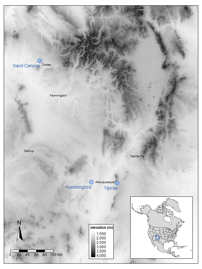
tmap_save(full_map, "Figure 1.jpg", dpi = 300, insets_tm = north_am_map,
          insets_vp = vp, height = 4.6, width = 3.5, units = "in")
3 Figure 2
Plant genera reported by Scribner and Krysl (1982) were assigned a photosynthetic pathway from the following sources: Basinger and Robertson (1997), Bruhl and Wilson (2007), Danneberger (1999), Giussani et al. (2001), Kocacinar and Sage (2003), Nelson (2012), Osborne et al. (2014), and Syvertsen et al. (1976).
Table_2 <- read.csv("Scribner and Krysl_Table 2/Table 2.csv", header = TRUE)

Pathway <- Table_2 %>%
  dplyr::select(Environmental.Context, Photosynthetic.pathway, DF....) %>%
  group_by(Environmental.Context, Photosynthetic.pathway) %>%
  summarize(sum_DF = sum(DF....), .groups = "keep")

labels <- c("Agricultural Playa Basins" = "Agricultural Context",
            "Playa Basins" = "Non-Agricultural Context")

Pathway %>%
ggplot(aes(x = reorder(Photosynthetic.pathway, -sum_DF), y = sum_DF)) +
  geom_bar(stat = "identity", linewidth = 0.75, alpha = 0.5, color = "#4d4d4d") +
  facet_wrap(~ Environmental.Context, ncol = 2,
             labeller = labeller(Environmental.Context = labels)) +
  scale_x_discrete(labels = parse(text = c("C[4]", "C[3]", "C[3]/C[4]"))) +
  theme_classic() +
  theme(legend.position="none",
        strip.background = element_blank(),
        strip.text.x = element_text(color = "#4d4d4d", size = 12,
                                    face = "bold"),
        axis.line = element_line(color = "#4d4d4d", linewidth = 0.75),
        axis.text.x = element_text(color = "#4d4d4d", size = 10),
        axis.text.y = element_text(color = "#4d4d4d", size = 10),
        axis.title.x = element_text(color = "#4d4d4d", size = 12,
                                    face = "bold"),
        axis.title.y = element_text(color = "#4d4d4d", size = 12,
                                    face = "bold"),
        axis.ticks.x = element_line(color = "#4d4d4d", linewidth = 0.75),
        axis.ticks.y = element_line(color = "#4d4d4d", linewidth = 0.75)) +
        labs(x = "Photosynthetic Pathway", y = "% Diet")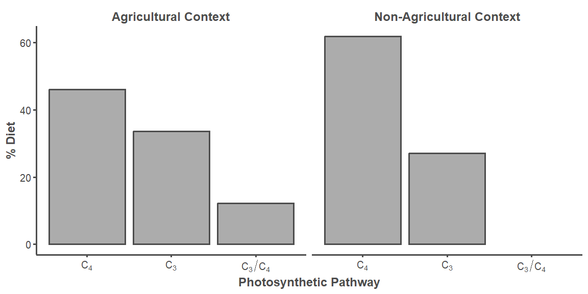
ggsave("Figure 2.jpg", dpi = 300, height = 4, width = 8)4 Isotope Data
We demineralized bone from the archaeo dataset in 0.5 N hydrochloric acid, removed lipids using 2:1 chloroform:methanol, and freeze-dried the resulting collagen pseudomorph overnight. We weighed out between 0.5 and 0.6 mg of collagen for the analysis of δ13C and δ15N. All seeds from the seeds dataset were purchased from Native seeds/SEARCH. We used between 5.0 and 6.0 mg of ground corn and 2.0 and 2.5 mg of ground bean/squash for the analysis of δ13C and δ15N. δ13C and δ15N were measured at the University of New Mexico Center for Stable Isotopes (UNM CSI, Albuquerque, NM) on a Thermo Scientific Delta V isotope ratio mass spectrometer (IRMS) with a dual inlet and Conflo IV interface coupled to a Costech 4010 elemental analyzer (EA). Stable isotope values are reported as parts per mil (‰).
The humans and turkeys isotope values come from the following sources: Chisholm and Matson (1994), Coltrain, Janetski, and Carlyle (2007), Conrad et al. (2016), Jones et al. (2016), Kellner et al. (2010), Kennett et al. (2017), Martin (1999), McCaffery et al. (2014), and Rawlings and Driver (2010).
archaeo <- read.csv("archaeological.csv", header = TRUE)
seeds <- read.csv("modern seeds.csv", header = TRUE)
turkeys <- read.csv("turkeys.csv", header = TRUE)
humans <- read.csv("humans.csv", header = TRUE)
5 Assessing Collagen Purity
Boxplots of C:Natomic values of archaeological leporid collagen per site. The blue box represents the acceptable range of collagen purity (2.9-3.6) reported by Ambrose (1990).
archaeo %>%
  mutate(CNatomic = CN * (14/12)) %>%
  ggplot(mapping = aes(y = CNatomic, x = Site.Name, group = Site.Name)) +
  geom_boxplot(color = "#4d4d4d", linewidth = 0.75) +
  labs(y = expression("C:N"[atomic]), x = "Archaeological Site") +
  theme_classic() +
  theme(legend.position="none",
        axis.line = element_line(color = "#4d4d4d", linewidth = 1),
        axis.text.x = element_text(color = "#4d4d4d", size = 12),
        axis.text.y = element_text(color = "#4d4d4d", size = 12),
        axis.title.x = element_text(color = "#4d4d4d", size = 14),
        axis.title.y = element_text(color = "#4d4d4d", size = 14),
        axis.ticks.x = element_line(color = "#4d4d4d", linewidth = 1),
        axis.ticks.y = element_line(color = "#4d4d4d", linewidth = 1)) +
    scale_y_continuous(limits=c(2.9, 3.6)) +
  annotate(geom = "rect", xmin = -Inf, xmax = Inf, ymin = 2.9, ymax = 3.6,
           color = "#5da5d8", fill =  "#5da5d8", alpha = 0.5, linewidth = 1)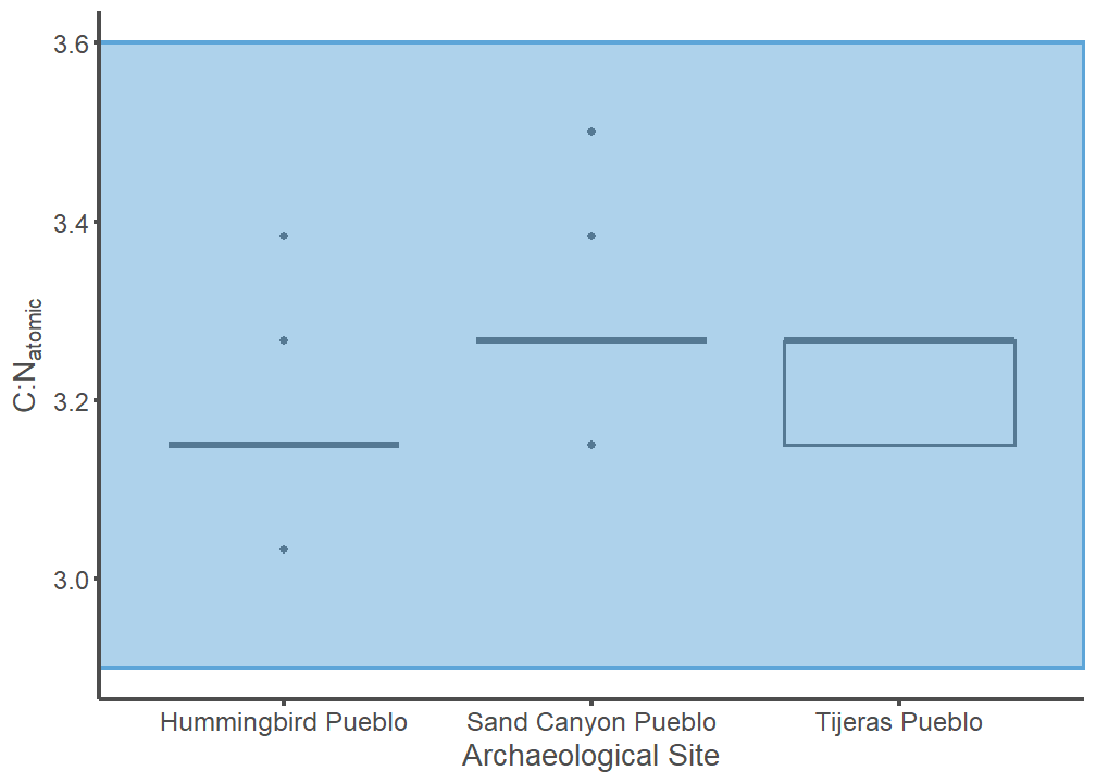
6 Data Wrangling
A 13C Suess correction of 2.0‰ was applied to the modern seed data (Dombrosky 2020).
seeds <- seeds %>%
  mutate(d13Csuess = d13C + 2)

archaeo_SIBER <- archaeo %>%
  unite(group, Site.Name, Genus, sep = " ") %>%
  dplyr::select(group, d13C, d15N)

seeds_SIBER <- seeds %>%
  dplyr::select(Comparative.Group, d13Csuess, d15N) %>%
  rename(group = Comparative.Group,
         d13C = d13Csuess)

turkeys_SIBER <- turkeys %>%
  mutate(animal = "Turkey") %>%
  unite(group, Diet.Type, animal, sep = " ") %>%
  dplyr::select(group, d13C, d15N)


humans_SIBER <-  humans %>%
  mutate(group = "Humans") %>%
  dplyr::select(group, d13C, d15N)

SIBER_data <- rbind(archaeo_SIBER, seeds_SIBER, turkeys_SIBER, humans_SIBER)
7 Figure 3
7.1 Sand Canyon Pueblo Figures
sand_label_df <- data.frame(
group = c("Sand Canyon Pueblo Lepus", "Sand Canyon Pueblo Sylvilagus",
"Free-ranging Turkey", "Humans", "Maize-fed Turkey", "Bean",
"Squash", "Corn"),
label = c("Sand Canyon Pueblo\nJackrabbbits",
"Sand Canyon Pueblo\nCottontails",
"Free-Ranging\nTurkeys", "Humans", "Maize-Fed Turkeys", "Beans",
"Squash", "Maize"),
d13C = c(-17, -20, -13.25, -5.8, -8, -25.25, -24, -9.75),
d15N = c(-0.75, 11, 2.5, 12.2, 4.1, -2, 13.25, -1),
hjust = c(0.5, 0.5, 0.5, 0, 0, 1, 1, 1),
vjust = c(1, 0, 0, 1, 1, 1, 0, 1))
sand_label_df$group <- factor(sand_label_df$group,
levels = c("Sand Canyon Pueblo Lepus",
"Sand Canyon Pueblo Sylvilagus",
"Free-ranging Turkey", "Humans",
"Maize-fed Turkey", "Bean", "Squash",
"Corn"))
sand_plot <- SIBER_data %>%
filter(group %in% c("Sand Canyon Pueblo Lepus",
"Sand Canyon Pueblo Sylvilagus",
"Bean", "Corn", "Squash", "Free-ranging Turkey",
"Maize-fed Turkey", "Humans"))
sand_plot$group <- factor(sand_plot$group,
levels = c("Sand Canyon Pueblo Lepus",
"Sand Canyon Pueblo Sylvilagus",
"Free-ranging Turkey", "Humans",
"Maize-fed Turkey", "Bean", "Squash",
"Corn"))
sand_p1 <- ggplot(sand_plot, aes(x = d13C, y = d15N)) +
geom_point(aes(fill = group, color = group), stroke = 1, size = 4,
alpha = 0.5, shape = 21) +
geom_point(aes(color = group), fill = NA, stroke = 1, size = 4,
shape = 21) +
labs(x = "δ<sup>13</sup>C (‰)",
y = "δ<sup>15</sup>N (‰)") +
theme_classic() +
theme(legend.position = "none",
axis.line = element_line(color = "#4d4d4d", linewidth = 1),
axis.text.x = element_text(color = "#4d4d4d", size = 12),
axis.text.y = element_text(color = "#4d4d4d", size = 12),
axis.title.x = element_markdown(color = "#4d4d4d", size = 14,
face = "bold"),
axis.title.y = element_markdown(color = "#4d4d4d", size = 14,
face = "bold"),
axis.ticks.x = element_line(color = "#4d4d4d", linewidth = 1),
axis.ticks.y = element_line(color = "#4d4d4d", linewidth = 1)) +
scale_color_viridis_d() +
stat_ellipse(aes(group = interaction(group), color = group, fill = group),
alpha = 0.25, linewidth = 0.75, linetype = 3, level = 0.95,
type = "t", geom = "polygon") +
geom_text(data = sand_label_df,aes(x = d13C, y = d15N,
label = label, color = group, hjust = hjust,
vjust = vjust),
size = 10/.pt, fontface = "bold") +
scale_fill_viridis_d() +
scale_x_continuous(limits=c(-27.5, -4),
breaks = c(-25, -20, -15, -10, -5)) +
scale_y_continuous(limits=c(-3, 15))
sand_p1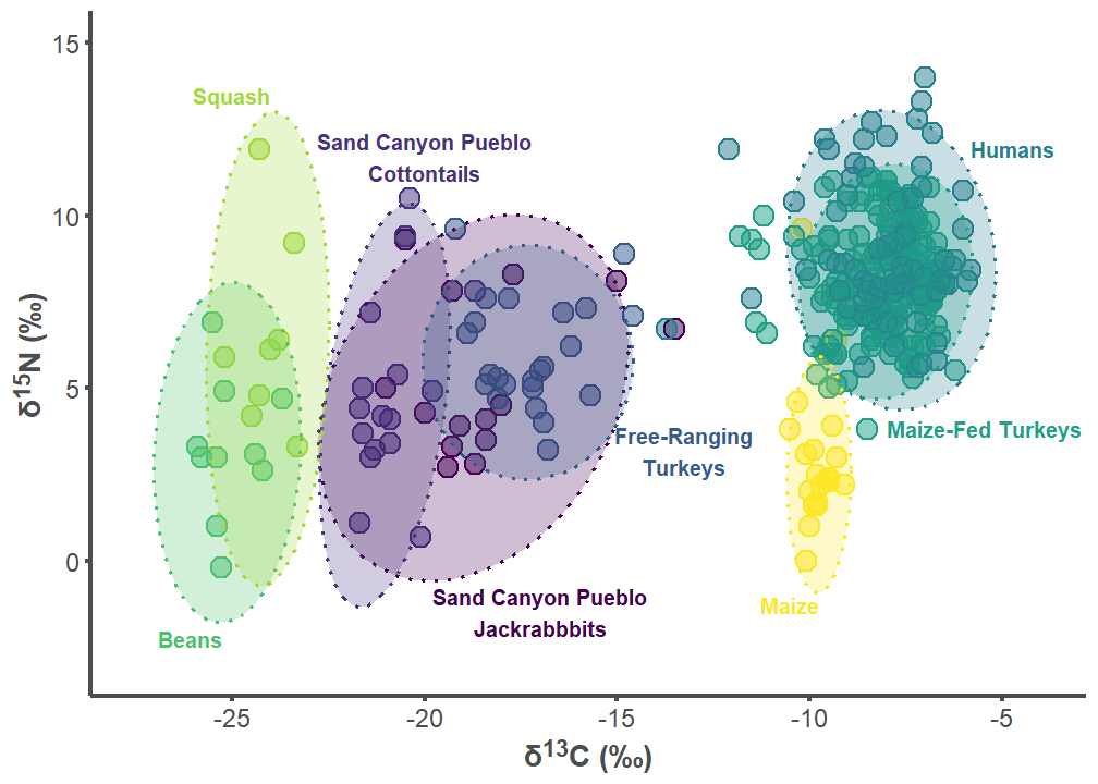
sand_p2 <- ggplot(sand_plot, aes(x = d13C, y = d15N)) +
labs(x = "δ<sup>13</sup>C (‰)",
y = "δ<sup>15</sup>N (‰)") +
theme_classic() +
theme(legend.position = "none",
axis.line = element_line(color = "#4d4d4d", linewidth = 1),
axis.text.x = element_text(color = "#4d4d4d", size = 12),
axis.text.y = element_text(color = "#4d4d4d", size = 12),
axis.title.x = element_markdown(color = "#4d4d4d", size = 14,
face = "bold"),
axis.title.y = element_markdown(color = "#4d4d4d", size = 14,
face = "bold"),
axis.ticks.x = element_line(color = "#4d4d4d", linewidth = 1),
axis.ticks.y = element_line(color = "#4d4d4d", linewidth = 1)) +
scale_color_viridis_d() +
stat_ellipse(aes(group = interaction(group), color = group, fill = group),
alpha = 0.5, linewidth = 1.1, linetype = 1, level = 0.40,
type = "t", geom = "polygon") +
stat_ellipse(aes(group = interaction(group), color = group, fill = group),
alpha = 0.25, linewidth = 0.75, linetype = 3, level = 0.95,
type = "t", geom = "polygon") +
geom_text(data = sand_label_df,aes(x = d13C, y = d15N,
label = label, color = group, hjust = hjust,
vjust = vjust),
size = 10/.pt, fontface = "bold") +
scale_fill_viridis_d() +
scale_x_continuous(limits=c(-27.5, -4),
breaks = c(-25, -20, -15, -10, -5)) +
scale_y_continuous(limits=c(-3, 15))
sand_p2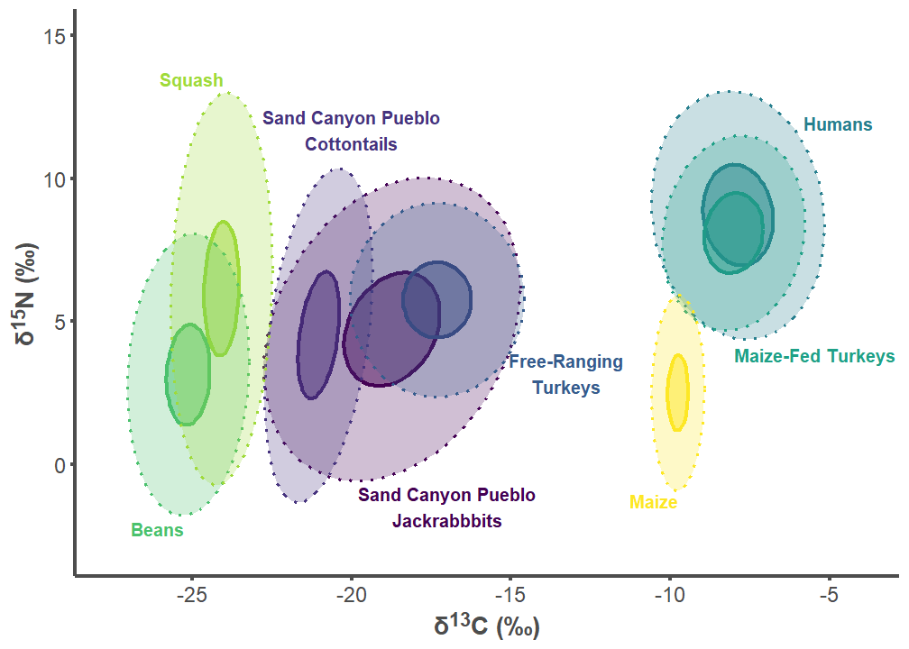
7.2 Hummingbird Pueblo Figures
hum_label_df <- data.frame(
group = c("Hummingbird Pueblo Lepus", "Hummingbird Pueblo Sylvilagus",
"Free-ranging Turkey", "Humans", "Maize-fed Turkey", "Bean",
"Squash", "Corn"),
label = c("Hummingbird Pueblo\nJackrabbbits",
"Hummingbird Pueblo\nCottontails",
"Free-Ranging\nTurkeys", "Humans", "Maize-Fed Turkeys", "Beans",
"Squash", "Maize"),
d13C = c(-20, -14.25, -20, -5.8, -8, -25.25, -24, -9.75),
d15N = c(1.5, -1.25, 10, 12.2, 4.1, -2, 13.25, -1),
hjust = c(0.5, 0.5, 0.5, 0, 0, 1, 1, 1),
vjust = c(1, 0, 0, 1, 1, 1, 0, 1))
hum_label_df$group <- factor(hum_label_df$group,
levels = c("Hummingbird Pueblo Lepus",
"Hummingbird Pueblo Sylvilagus",
"Free-ranging Turkey", "Humans",
"Maize-fed Turkey", "Bean", "Squash",
"Corn"))
hum_plot <- SIBER_data %>%
filter(group %in% c("Hummingbird Pueblo Lepus",
"Hummingbird Pueblo Sylvilagus",
"Bean", "Corn", "Squash", "Free-ranging Turkey",
"Maize-fed Turkey", "Humans"))
hum_plot$group <- factor(hum_plot$group,
levels = c("Hummingbird Pueblo Lepus",
"Hummingbird Pueblo Sylvilagus",
"Free-ranging Turkey", "Humans",
"Maize-fed Turkey", "Bean", "Squash",
"Corn"))
hum_p1 <- ggplot(hum_plot, aes(x = d13C, y = d15N)) +
geom_point(aes(fill = group, color = group), stroke = 1, size = 4,
alpha = 0.5, shape = 21) +
geom_point(aes(color = group), fill = NA, stroke = 1, size = 4,
shape = 21) +
labs(x = "δ<sup>13</sup>C (‰)",
y = "δ<sup>15</sup>N (‰)") +
theme_classic() +
theme(legend.position = "none",
axis.line = element_line(color = "#4d4d4d", linewidth = 1),
axis.text.x = element_text(color = "#4d4d4d", size = 12),
axis.text.y = element_text(color = "#4d4d4d", size = 12),
axis.title.x = element_markdown(color = "#4d4d4d", size = 14,
face = "bold"),
axis.title.y = element_markdown(color = "#4d4d4d", size = 14,
face = "bold"),
axis.ticks.x = element_line(color = "#4d4d4d", linewidth = 1),
axis.ticks.y = element_line(color = "#4d4d4d", linewidth = 1)) +
scale_color_viridis_d() +
stat_ellipse(aes(group = interaction(group), color = group, fill = group),
alpha = 0.25, linewidth = 0.75, linetype = 3, level = 0.95,
type = "t", geom = "polygon") +
geom_text(data = hum_label_df,aes(x = d13C, y = d15N,
label = label, color = group, hjust = hjust,
vjust = vjust),
size = 10/.pt, fontface = "bold") +
scale_fill_viridis_d() +
scale_x_continuous(limits=c(-27.5, -4),
breaks = c(-25, -20, -15, -10, -5)) +
scale_y_continuous(limits=c(-3, 15))
hum_p1
hum_p2 <- ggplot(hum_plot, aes(x = d13C, y = d15N)) +
labs(x = "δ<sup>13</sup>C (‰)",
y = "δ<sup>15</sup>N (‰)") +
theme_classic() +
theme(legend.position = "none",
axis.line = element_line(color = "#4d4d4d", linewidth = 1),
axis.text.x = element_text(color = "#4d4d4d", size = 12),
axis.text.y = element_text(color = "#4d4d4d", size = 12),
axis.title.x = element_markdown(color = "#4d4d4d", size = 14,
face = "bold"),
axis.title.y = element_markdown(color = "#4d4d4d", size = 14,
face = "bold"),
axis.ticks.x = element_line(color = "#4d4d4d", linewidth = 1),
axis.ticks.y = element_line(color = "#4d4d4d", linewidth = 1)) +
scale_color_viridis_d() +
stat_ellipse(aes(group = interaction(group), color = group, fill = group),
alpha = 0.5, linewidth = 1.1, linetype = 1, level = 0.40, type = "t",
geom = "polygon") +
stat_ellipse(aes(group = interaction(group), color = group, fill = group),
alpha = 0.25, linewidth = 0.75, linetype = 3, level = 0.95,
type = "t", geom = "polygon") +
geom_text(data = hum_label_df,aes(x = d13C, y = d15N,
label = label, color = group, hjust = hjust,
vjust = vjust),
size = 10/.pt, fontface = "bold") +
scale_fill_viridis_d() +
scale_x_continuous(limits=c(-27.5, -4),
breaks = c(-25, -20, -15, -10, -5)) +
scale_y_continuous(limits=c(-3, 15))
hum_p2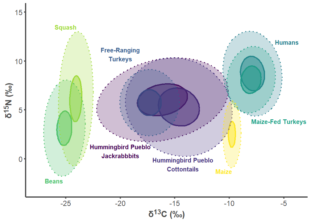
7.3 Tijeras Pueblo Figures
tij_label_df <- data.frame(
group = c("Tijeras Pueblo Lepus", "Tijeras Pueblo Sylvilagus",
"Free-ranging Turkey", "Humans", "Maize-fed Turkey", "Bean",
"Squash", "Corn"),
label = c("Tijeras Pueblo\nJackrabbbits",
"Tijeras Pueblo\nCottontails",
"Free-Ranging\nTurkeys", "Humans", "Maize-Fed Turkeys", "Beans",
"Squash", "Maize"),
d13C = c(-21, -17.5, -17.25, -5.8, -8, -25.25, -24, -9.75),
d15N = c(1.5, -1.75, 9.5, 12.2, 4.1, -2, 13.25, -1),
hjust = c(0.5, 0.5, 0.5, 0, 0, 1, 1, 1),
vjust = c(1, 0, 0, 1, 1, 1, 0, 1))
tij_label_df$group <- factor(tij_label_df$group,
levels = c("Tijeras Pueblo Lepus",
"Tijeras Pueblo Sylvilagus",
"Free-ranging Turkey", "Humans",
"Maize-fed Turkey", "Bean", "Squash",
"Corn"))
tij_plot <- SIBER_data %>%
filter(group %in% c("Tijeras Pueblo Lepus",
"Tijeras Pueblo Sylvilagus",
"Bean", "Corn", "Squash", "Free-ranging Turkey",
"Maize-fed Turkey", "Humans"))
tij_plot$group <- factor(tij_plot$group,
levels = c("Tijeras Pueblo Lepus",
"Tijeras Pueblo Sylvilagus",
"Free-ranging Turkey", "Humans",
"Maize-fed Turkey", "Bean", "Squash",
"Corn"))
tij_p1 <- ggplot(tij_plot, aes(x = d13C, y = d15N)) +
geom_point(aes(fill = group, color = group), stroke = 1, size = 4,
alpha = 0.5, shape = 21) +
geom_point(aes(color = group), fill = NA, stroke = 1, size = 4,
shape = 21) +
labs(x = "δ<sup>13</sup>C (‰)",
y = "δ<sup>15</sup>N (‰)") +
theme_classic() +
theme(legend.position = "none",
axis.line = element_line(color = "#4d4d4d", linewidth = 1),
axis.text.x = element_text(color = "#4d4d4d", size = 12),
axis.text.y = element_text(color = "#4d4d4d", size = 12),
axis.title.x = element_markdown(color = "#4d4d4d", size = 14,
face = "bold"),
axis.title.y = element_markdown(color = "#4d4d4d", size = 14,
face = "bold"),
axis.ticks.x = element_line(color = "#4d4d4d", linewidth = 1),
axis.ticks.y = element_line(color = "#4d4d4d", linewidth = 1)) +
scale_color_viridis_d() +
stat_ellipse(aes(group = interaction(group), color = group, fill = group),
alpha = 0.25, linewidth = 0.75, linetype = 3, level = 0.95,
type = "t", geom = "polygon") +
geom_text(data = tij_label_df,aes(x = d13C, y = d15N,
label = label, color = group, hjust = hjust,
vjust = vjust),
size = 10/.pt, fontface = "bold") +
scale_fill_viridis_d() +
scale_x_continuous(limits=c(-27.5, -4),
breaks = c(-25, -20, -15, -10, -5)) +
scale_y_continuous(limits=c(-3, 15))
tij_p1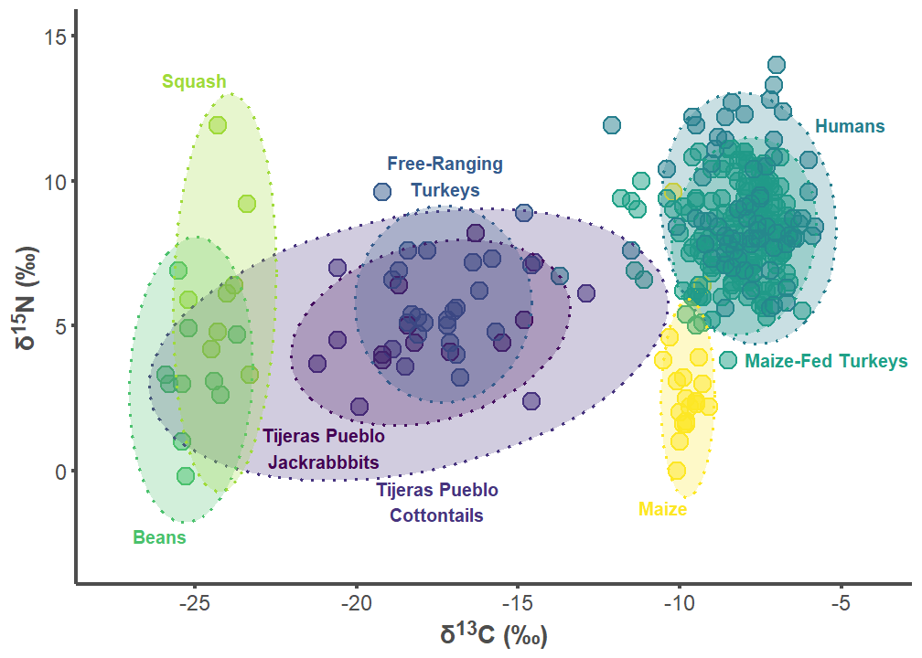
tij_p2 <- ggplot(tij_plot, aes(x = d13C, y = d15N)) +
labs(x = "δ<sup>13</sup>C (‰)",
y = "δ<sup>15</sup>N (‰)") +
theme_classic() +
theme(legend.position = "none",
axis.line = element_line(color = "#4d4d4d", linewidth = 1),
axis.text.x = element_text(color = "#4d4d4d", size = 12),
axis.text.y = element_text(color = "#4d4d4d", size = 12),
axis.title.x = element_markdown(color = "#4d4d4d", size = 14,
face = "bold"),
axis.title.y = element_markdown(color = "#4d4d4d", size = 14,
face = "bold"),
axis.ticks.x = element_line(color = "#4d4d4d", linewidth = 1),
axis.ticks.y = element_line(color = "#4d4d4d", linewidth = 1)) +
scale_color_viridis_d() +
stat_ellipse(aes(group = interaction(group), color = group, fill = group),
alpha = 0.5, linewidth = 1.1, linetype = 1, level = 0.40,
type = "t", geom = "polygon") +
stat_ellipse(aes(group = interaction(group), color = group, fill = group),
alpha = 0.25, linewidth = 0.75, linetype = 3, level = 0.95,
type = "t", geom = "polygon") +
geom_text(data = tij_label_df,aes(x = d13C, y = d15N,
label = label, color = group, hjust = hjust,
vjust = vjust),
size = 10/.pt, fontface = "bold") +
scale_fill_viridis_d() +
scale_x_continuous(limits=c(-27.5, -4),
breaks = c(-25, -20, -15, -10, -5)) +
scale_y_continuous(limits=c(-3, 15))
tij_p2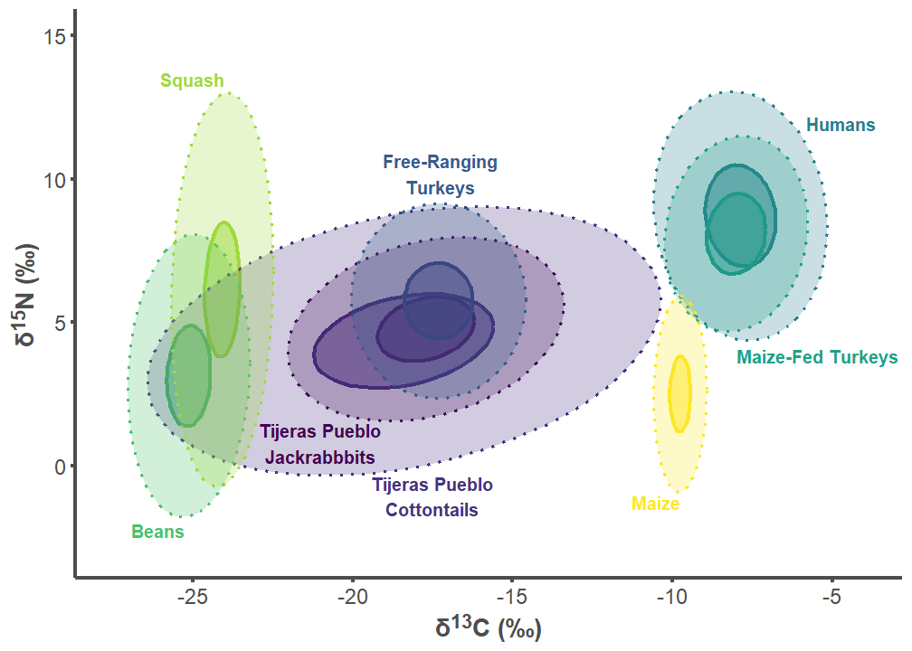
7.4 Combine Figures
all_plots <- plot_grid(sand_p1, sand_p2, hum_p1, hum_p2, tij_p1, tij_p2,
                       labels = "AUTO", label_colour = "#4d4d4d",
                       label_size = 20, ncol = 2, nrow = 3)

all_plots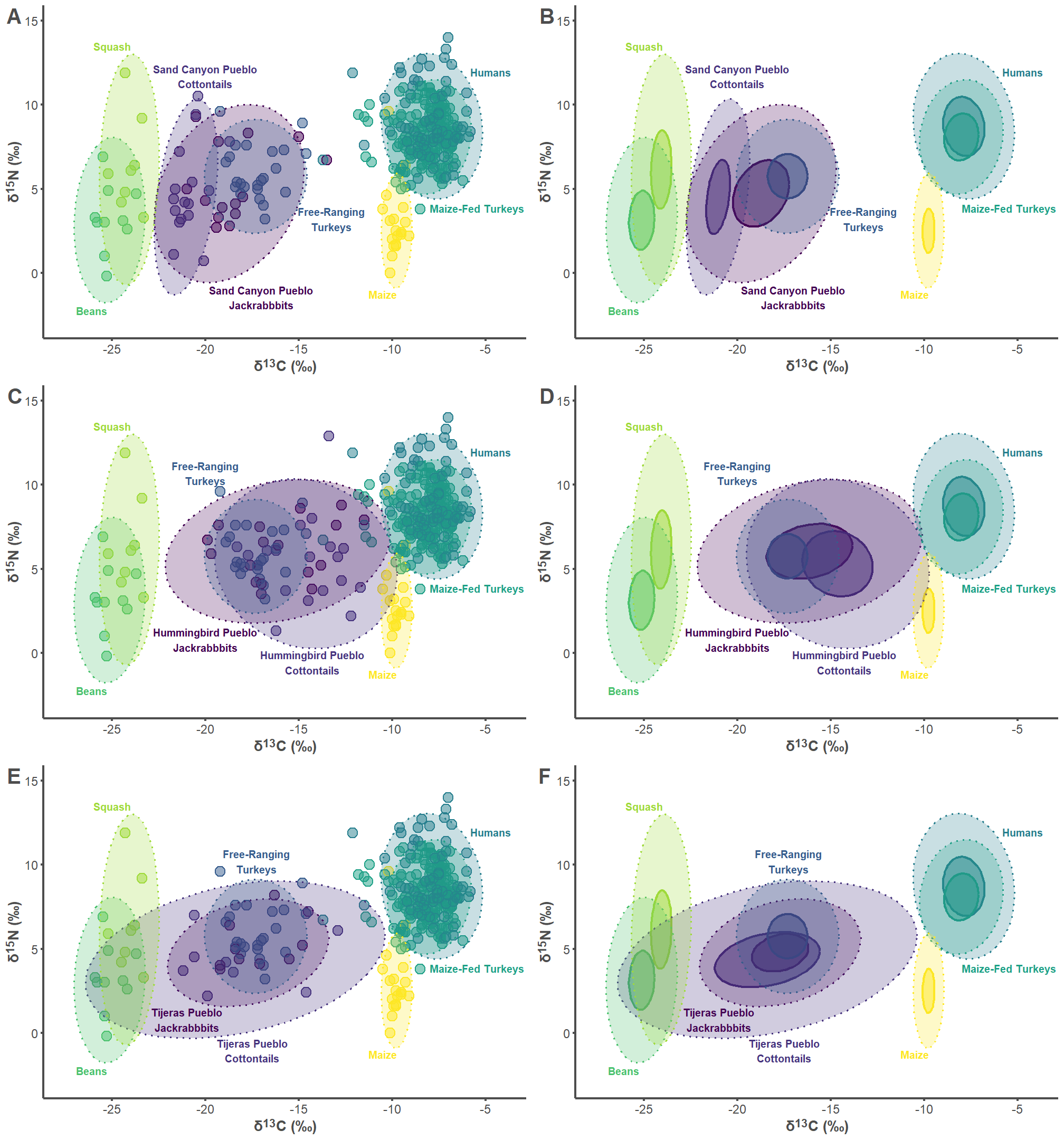
ggsave("Figure 3.jpg", dpi = 300, height = 15, width = 14)8 Ellipse Area Calculations
8.1 Functions
This function is to summarize p-values in tables. Scientific notation is too long.
p_val_format <- function(x){
  z <- scales::pvalue_format()(x)
  z[!is.finite(x)] <- ""
  z
}
8.2 Test for Normality
Some isotope values per group are non-normal. Thus, ellipses in Figure 2 are visualized based on the t-distribution, which is also good for small sample sizes.
SIBER_data %>%
  group_by(group) %>%
  do(tidy(shapiro.test(.$d13C))) %>%
  dplyr::select(group, statistic, p.value) %>%
  ungroup() %>%
  gt() %>%
  fmt(columns = p.value,
      fns = p_val_format) %>%
  fmt_number(columns = statistic, decimals = 2) %>%
  cols_label(group = md("**Group**"),
             statistic = md("***W* Statistic**"),
             p.value = md("**P-Value**")) %>%
tab_header(title = html("<b>δ<sup>13</sup>C Normality</b>"))| δ13C Normality | ||
| Group | W Statistic | P-Value |
|---|---|---|
| Bean | 0.88 | 0.139 |
| Corn | 0.98 | 0.928 |
| Free-ranging Turkey | 0.96 | 0.462 |
| Humans | 0.91 | <0.001 |
| Hummingbird Pueblo Lepus | 0.96 | 0.565 |
| Hummingbird Pueblo Sylvilagus | 0.96 | 0.502 |
| Maize-fed Turkey | 0.94 | <0.001 |
| Sand Canyon Pueblo Lepus | 0.86 | 0.033 |
| Sand Canyon Pueblo Sylvilagus | 0.88 | 0.041 |
| Squash | 0.96 | 0.788 |
| Tijeras Pueblo Lepus | 0.90 | 0.251 |
| Tijeras Pueblo Sylvilagus | 0.86 | 0.088 |
SIBER_data %>%
  group_by(group) %>%
  do(tidy(shapiro.test(.$d15N))) %>%
  dplyr::select(group, statistic, p.value) %>%
  ungroup() %>%
  gt() %>%
  fmt(columns = p.value,
      fns = p_val_format) %>%
  fmt_number(columns = statistic, decimals = 2) %>%
  cols_label(group = md("**Group**"),
             statistic = md("***W* Statistic**"),
             p.value = md("**P-Value**")) %>%
tab_header(title = html("<b>δ<sup>15</sup>N Normality</b>"))| δ15N Normality | ||
| Group | W Statistic | P-Value |
|---|---|---|
| Bean | 0.96 | 0.766 |
| Corn | 0.82 | 0.002 |
| Free-ranging Turkey | 0.96 | 0.462 |
| Humans | 0.94 | 0.002 |
| Hummingbird Pueblo Lepus | 0.95 | 0.390 |
| Hummingbird Pueblo Sylvilagus | 0.90 | 0.050 |
| Maize-fed Turkey | 0.99 | 0.079 |
| Sand Canyon Pueblo Lepus | 0.88 | 0.066 |
| Sand Canyon Pueblo Sylvilagus | 0.94 | 0.376 |
| Squash | 0.90 | 0.314 |
| Tijeras Pueblo Lepus | 0.82 | 0.035 |
| Tijeras Pueblo Sylvilagus | 0.92 | 0.371 |
8.3 SIBER Area Calculations
TA = Total Area, SEA = Standard Ellipse Area, and SEAc = Small Sample Size Corrected Standard Ellipse Area (Jackson et al. 2011).
siber.example <- SIBER_data %>%
  dplyr::select(d13C, d15N, group) %>%
  mutate(community = 1) %>%
  rename(iso1 = d13C,
         iso2 = d15N)

siber.example <- createSiberObject(siber.example)

group.ML1 <- data.frame(groupMetricsML(siber.example)) %>%
  rename("Hummingbird Jackrabbits" = X1.Hummingbird.Pueblo.Lepus,
         "Hummingbird Cottontails" = X1.Hummingbird.Pueblo.Sylvilagus,
         "Sand Canyon Jackrabbit" = X1.Sand.Canyon.Pueblo.Lepus,
         "Sand Canyon Cottontails" = X1.Sand.Canyon.Pueblo.Sylvilagus,
         "Tijeras Pueblo Jackrabbits" = X1.Tijeras.Pueblo.Lepus,
         "Tijeras Pueblo Cottontails" = X1.Tijeras.Pueblo.Sylvilagus,
         "Beans" = X1.Bean,
         "Maize" = X1.Corn,
         "Squash" = X1.Squash,
         "Free-ranging Turkeys" = X1.Free.ranging.Turkey,
         "Maize-fed Turkeys" = X1.Maize.fed.Turkey,
         "Humans" = X1.Humans) %>%
  t() %>%
  round(digits = 2)

group.ML1 %>%
  data.frame() %>%
  rownames_to_column() %>%
  rename(group = rowname) %>%
  gt() %>%
  cols_label(group = md("**Group**"),
             TA = md("**TA**"),
             SEA = md("**SEA**"),
             SEAc = html("<b>SEA<sub>c</sub></b>")) %>%
  tab_header(title = md("**SIBER Area Calculations**")) %>%
  tab_footnote(
    footnote = html("All values are ‰<sup>2</sup>"),
locations = cells_title(groups = "title"))| SIBER Area Calculations1 | |||
| Group | TA | SEA | SEAc |
|---|---|---|---|
| Hummingbird Jackrabbits | 28.91 | 13.02 | 13.88 |
| Hummingbird Cottontails | 44.81 | 15.47 | 16.38 |
| Sand Canyon Jackrabbit | 29.74 | 13.82 | 14.97 |
| Sand Canyon Cottontails | 18.75 | 6.43 | 6.89 |
| Tijeras Pueblo Cottontails | 33.91 | 17.58 | 20.09 |
| Tijeras Pueblo Jackrabbits | 11.71 | 7.01 | 8.01 |
| Beans | 8.41 | 4.53 | 5.10 |
| Maize | 8.21 | 2.40 | 2.53 |
| Squash | 10.09 | 5.47 | 6.38 |
| Free-ranging Turkeys | 19.40 | 6.16 | 6.46 |
| Maize-fed Turkeys | 28.55 | 5.19 | 5.22 |
| Humans | 46.75 | 8.81 | 8.93 |
| 1 All values are ‰2 | |||
8.4 Table 1
SIBER Maximum Likelihood Overlap with Humans Calculations
samp_size <- data.frame(siber.example[["sample.sizes"]]) %>%
  rename("Hummingbird Pueblo Jackrabbits" = Hummingbird.Pueblo.Lepus,
         "Hummingbird Pueblo Cottontails" = Hummingbird.Pueblo.Sylvilagus,
         "Sand Canyon Pueblo Jackrabbits" = Sand.Canyon.Pueblo.Lepus,
         "Sand Canyon Pueblo Cottontails" = Sand.Canyon.Pueblo.Sylvilagus,
         "Tijeras Pueblo Jackrabbits" = Tijeras.Pueblo.Lepus,
         "Tijeras Pueblo Cottontails" = Tijeras.Pueblo.Sylvilagus,
         "Beans" = Bean,
         "Maize" = Corn,
         "Squash" = Squash,
         "Free-ranging Turkeys" = Free.ranging.Turkey,
         "Maize-fed Turkeys" = Maize.fed.Turkey,
         "Humans" = Humans) %>%
  pivot_longer(cols = 1:12, names_to = "group", values_to = "n")
results <- data.frame()
taxa <- c("1.Sand Canyon Pueblo Lepus", "1.Sand Canyon Pueblo Sylvilagus",
"1.Hummingbird Pueblo Lepus", "1.Hummingbird Pueblo Sylvilagus",
"1.Tijeras Pueblo Lepus",
"1.Tijeras Pueblo Sylvilagus",
"1.Maize-fed Turkey")
for (i in seq_along(taxa)) {
sea.overlap <- maxLikOverlap(taxa[[i]], "1.Humans", siber.example,
p.interval = 0.95, n = 100)
results[i, 1] <- taxa[[i]]
results[i, 2] <- round(sea.overlap[[3]], digits = 2)
results[i, 3] <- round(sea.overlap[[3]]/sea.overlap[[2]]*100, digits = 2)
results[i, 4] <- round(sea.overlap[[3]]/sea.overlap[[1]]*100, digits = 2)
results[i, 5] <- round(sea.overlap[[3]]/(sea.overlap[[2]] +
sea.overlap[[1]] -
sea.overlap[[3]])*100, digits = 2)
}
colnames(results) <- c("group", "overlap ‰", "% human niche", "% group niche",
"% overlap")
results$group <- gsub("1.","", as.character(results$group))
results$group <- gsub("Lepus","Jackrabbits", as.character(results$group))
results$group <- gsub("Sylvilagus","Cottontails", as.character(results$group))
results$group <- gsub("Turkey","Turkeys", as.character(results$group))
results %>%
left_join(., samp_size, by = "group") %>%
dplyr::select(group, n, `overlap ‰`, `% human niche`, `% group niche`,
`% overlap`) %>%
gt() %>%
cols_label(group = md("**Group**"),
n = md("**n**"),
"overlap ‰" = html("<b>Overlap ‰<sup>2</sup></b>"),
"% human niche" = md("**% Human Niche**"),
"% group niche" = md("**% Group's Niche**"),
"% overlap" = md("**% Overlap**")) %>%
tab_header(title = md("**Human Isotopic Niche Overlap Calculations**")) %>%
tab_footnote(
footnote = "Proportion of overlap relative to non-overlapping area.",
locations = cells_column_labels(columns = "% overlap")
)| Human Isotopic Niche Overlap Calculations | |||||
| Group | n | Overlap ‰2 | % Human Niche | % Group’s Niche | % Overlap1 |
|---|---|---|---|---|---|
| Sand Canyon Pueblo Jackrabbits | 14 | 0.00 | 0.00 | 0.00 | 0.00 |
| Sand Canyon Pueblo Cottontails | 16 | 0.00 | 0.00 | 0.00 | 0.00 |
| Hummingbird Pueblo Jackrabbits | 17 | 4.55 | 8.50 | 5.47 | 3.44 |
| Hummingbird Pueblo Cottontails | 19 | 4.61 | 8.62 | 4.70 | 3.14 |
| Tijeras Pueblo Jackrabbits | 9 | 0.00 | 0.00 | 0.00 | 0.00 |
| Tijeras Pueblo Cottontails | 9 | 2.38 | 4.45 | 1.98 | 1.39 |
| Maize-fed Turkeys | 180 | 31.23 | 58.39 | 100.00 | 58.39 |
| 1 Proportion of overlap relative to non-overlapping area. | |||||
round(mean(results$`% human niche`[1:6]), digits = 2)[1] 3.59round(mean(results$`% group niche`[1:6]), digits = 2)[1] 2.029 Figure 4
This example uses functional programming instead of the above for loop.
set.seed(4611)

# options for running jags
parms <- list()
parms$n.iter <- 2 * 10^4
parms$n.burnin <- 1 * 10^3
parms$n.thin <- 10
parms$n.chains <- 2

# define the priors
priors <- list()
priors$R <- 1 * diag(2)
priors$k <- 2
priors$tau.mu <- 1.0E-3

ellipses.posterior <- siberMVN(siber.example, parms, priors)
bayes95.overlap <- function(x) bayesianOverlap(x, "1.Humans",
ellipses.posterior, draws = 1000,
p.interval = 0.95, n = 100)set.seed(6809)
overlap_res <- taxa %>%
map_df(bayes95.overlap, .progress = TRUE) %>%
mutate(group = rep(c("Hummingbird Pueblo Jackrabbits",
"Hummingbird Pueblo Cottontails",
"Sand Canyon Pueblo Jackrabbits",
"Sand Canyon Pueblo Cottontails",
"Tijeras Pueblo Jackrabbits",
"Tijeras Pueblo Cottontails",
"Maize-fed Turkey"),
each = 1000))overlap_res$group <- factor(overlap_res$group,
levels = c("Sand Canyon Pueblo Jackrabbits",
"Sand Canyon Pueblo Cottontails",
"Hummingbird Pueblo Jackrabbits",
"Hummingbird Pueblo Cottontails",
"Tijeras Pueblo Jackrabbits",
"Tijeras Pueblo Cottontails",
"Maize-fed Turkey"))
overlap_res %>%
mutate(`% Overlap` = overlap / ((area1 + area2) - overlap) * 100) %>%
ggplot(aes(x = `% Overlap`, color = group, fill = group)) +
geom_histogram(binwidth = 2.5, alpha = 0.5) +
scale_fill_viridis_d() +
scale_color_viridis_d() +
scale_y_continuous(expand = c(0, 0)) +
scale_x_continuous(breaks = seq(0, 89, by = 10)) +
facet_wrap(~ group, ncol = 2) +
theme_classic() +
labs(x = "% Overlap", y = "Frequency") +
theme(legend.position = "none",
strip.background = element_blank())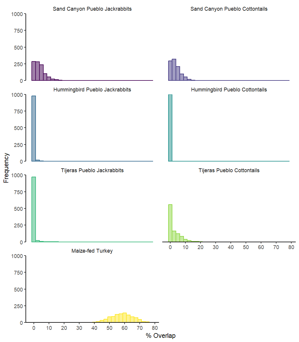
ggsave("Figure 4.jpg", dpi = 300, height = 8, width = 5)10 Trophic Discrimination Factors (TDFs)
We did not use TDFs in our analysis for a few different reasons. To our knowledge, there are no known feeding experiments using the amount of C4 resources that Ancestral Pueblo people relied on. Thus, all of the models developed to estimate TDFs based off diet quality do not capture this amount of variation. When we apply TDF models developed by Caut, Angulo, and Courchamp (2009) (see below) humans are projected into extremely unlikely carbon isotope space. Commonly relied on TDF estimation models appear to introduce more error than they help correct. Additionally, we see that these TDF-corrected values do not impact human-leporid overlap to any substantial degree. We argue that our reliance on 95% data ellipse overlap calculations (above) better incorporates error caused by trophic discrimination.
mammal <- c("Lepus", "Sylvilagus", "Human")

SIBER_data_tdf <- SIBER_data %>%
  mutate(d13C = case_when(str_detect(group, paste(mammal, collapse = "|")) ~
                           d13C - (-0.417 * d13C - 7.878),
                         str_detect(group, "Turkey") ~
                           d13C - (1.76 * 0.64), .default = d13C),
         new = case_when(str_detect(group, paste(mammal, collapse = "|")) ~
                           d15N - (-0.141 * d15N + 3.975),
                         str_detect(group, "Turkey") ~
                           d15N - (2.37 * 0.47), .default = d15N))
10.1 Sand Canyon TDF
sand_label_df <- data.frame(
group = c("Sand Canyon Pueblo Lepus", "Sand Canyon Pueblo Sylvilagus",
"Free-ranging Turkey", "Humans", "Maize-fed Turkey", "Bean",
"Squash", "Corn"),
label = c("Sand Canyon Pueblo\nJackrabbbits",
"Sand Canyon Pueblo\nCottontails",
"Free-Ranging\nTurkeys", "Humans", "Maize-Fed Turkeys", "Beans",
"Squash", "Maize"),
d13C = c(-17, -20, -13.25, -5.8, -8, -25.25, -24, -9.75),
d15N = c(-0.75, 11, 2.5, 12.2, 4.1, -2, 13.25, -1),
hjust = c(0.5, 0.5, 0.5, 0, 0, 1, 1, 1),
vjust = c(1, 0, 0, 1, 1, 1, 0, 1))
sand_label_df$group <- factor(sand_label_df$group,
levels = c("Sand Canyon Pueblo Lepus",
"Sand Canyon Pueblo Sylvilagus",
"Free-ranging Turkey", "Humans",
"Maize-fed Turkey", "Bean", "Squash",
"Corn"))
sand_plot <- SIBER_data_tdf %>%
filter(group %in% c("Sand Canyon Pueblo Lepus",
"Sand Canyon Pueblo Sylvilagus",
"Bean", "Corn", "Squash", "Free-ranging Turkey",
"Maize-fed Turkey", "Humans"))
sand_plot$group <- factor(sand_plot$group,
levels = c("Sand Canyon Pueblo Lepus",
"Sand Canyon Pueblo Sylvilagus",
"Free-ranging Turkey", "Humans",
"Maize-fed Turkey", "Bean", "Squash",
"Corn"))
sand_p1 <- ggplot(sand_plot, aes(x = d13C, y = d15N)) +
geom_point(aes(fill = group, color = group), stroke = 1, size = 4,
alpha = 0.5, shape = 21) +
geom_point(aes(color = group), fill = NA, stroke = 1, size = 4,
shape = 21) +
labs(x = "δ<sup>13</sup>C (‰)",
y = "δ<sup>15</sup>N (‰)") +
theme_classic() +
theme(legend.position = "none",
axis.line = element_line(color = "#4d4d4d", linewidth = 1),
axis.text.x = element_text(color = "#4d4d4d", size = 12),
axis.text.y = element_text(color = "#4d4d4d", size = 12),
axis.title.x = element_markdown(color = "#4d4d4d", size = 14,
face = "bold"),
axis.title.y = element_markdown(color = "#4d4d4d", size = 14,
face = "bold"),
axis.ticks.x = element_line(color = "#4d4d4d", linewidth = 1),
axis.ticks.y = element_line(color = "#4d4d4d", linewidth = 1)) +
scale_color_viridis_d() +
stat_ellipse(aes(group = interaction(group), color = group, fill = group),
alpha = 0.25, linewidth = 0.75, linetype = 3, level = 0.95,
type = "t", geom = "polygon") +
geom_text(data = sand_label_df,aes(x = d13C, y = d15N,
label = label, color = group, hjust = hjust,
vjust = vjust),
size = 10/.pt, fontface = "bold") +
scale_fill_viridis_d() +
scale_x_continuous(limits=c(-30, 5),
breaks = c(-30, -25, -20, -15, -10, -5, 0, 5)) +
scale_y_continuous(limits=c(-3, 15))
sand_p1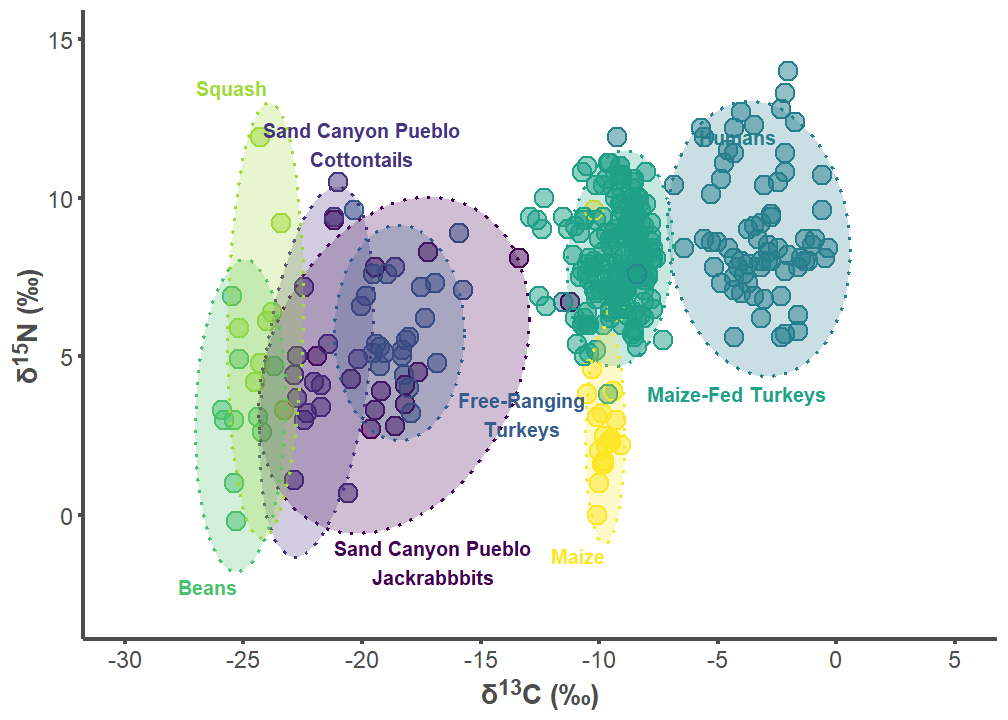
sand_p2 <- ggplot(sand_plot, aes(x = d13C, y = d15N)) +
labs(x = "δ<sup>13</sup>C (‰)",
y = "δ<sup>15</sup>N (‰)") +
theme_classic() +
theme(legend.position = "none",
axis.line = element_line(color = "#4d4d4d", linewidth = 1),
axis.text.x = element_text(color = "#4d4d4d", size = 12),
axis.text.y = element_text(color = "#4d4d4d", size = 12),
axis.title.x = element_markdown(color = "#4d4d4d", size = 14,
face = "bold"),
axis.title.y = element_markdown(color = "#4d4d4d", size = 14,
face = "bold"),
axis.ticks.x = element_line(color = "#4d4d4d", linewidth = 1),
axis.ticks.y = element_line(color = "#4d4d4d", linewidth = 1)) +
scale_color_viridis_d() +
stat_ellipse(aes(group = interaction(group), color = group, fill = group),
alpha = 0.5, linewidth = 1.1, linetype = 1, level = 0.40,
type = "t", geom = "polygon") +
stat_ellipse(aes(group = interaction(group), color = group, fill = group),
alpha = 0.25, linewidth = 0.75, linetype = 3, level = 0.95,
type = "t", geom = "polygon") +
geom_text(data = sand_label_df,aes(x = d13C, y = d15N,
label = label, color = group, hjust = hjust,
vjust = vjust),
size = 10/.pt, fontface = "bold") +
scale_fill_viridis_d() +
scale_x_continuous(limits=c(-30, 5),
breaks = c(-30, -25, -20, -15, -10, -5, 0, 5)) +
scale_y_continuous(limits=c(-3, 15))
sand_p2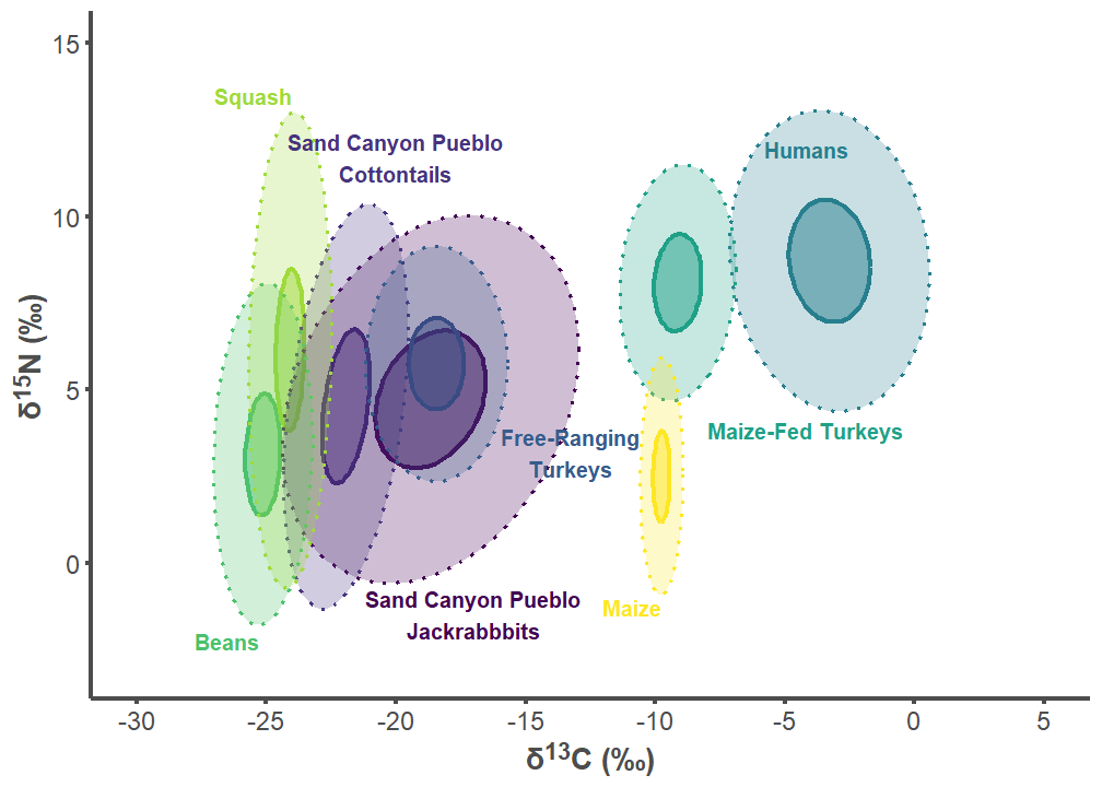
10.2 Hummingbird TDF
hum_label_df <- data.frame(
group = c("Hummingbird Pueblo Lepus", "Hummingbird Pueblo Sylvilagus",
"Free-ranging Turkey", "Humans", "Maize-fed Turkey", "Bean",
"Squash", "Corn"),
label = c("Hummingbird Pueblo\nJackrabbbits",
"Hummingbird Pueblo\nCottontails",
"Free-Ranging\nTurkeys", "Humans", "Maize-Fed Turkeys", "Beans",
"Squash", "Maize"),
d13C = c(-20, -14.25, -20, -5.8, -8, -25.25, -24, -9.75),
d15N = c(1.5, -1.25, 10, 12.2, 4.1, -2, 13.25, -1),
hjust = c(0.5, 0.5, 0.5, 0, 0, 1, 1, 1),
vjust = c(1, 0, 0, 1, 1, 1, 0, 1))
hum_label_df$group <- factor(hum_label_df$group,
levels = c("Hummingbird Pueblo Lepus",
"Hummingbird Pueblo Sylvilagus",
"Free-ranging Turkey", "Humans",
"Maize-fed Turkey", "Bean", "Squash",
"Corn"))
hum_plot <- SIBER_data_tdf %>%
filter(group %in% c("Hummingbird Pueblo Lepus",
"Hummingbird Pueblo Sylvilagus",
"Bean", "Corn", "Squash", "Free-ranging Turkey",
"Maize-fed Turkey", "Humans"))
hum_plot$group <- factor(hum_plot$group,
levels = c("Hummingbird Pueblo Lepus",
"Hummingbird Pueblo Sylvilagus",
"Free-ranging Turkey", "Humans",
"Maize-fed Turkey", "Bean", "Squash",
"Corn"))
hum_p1 <- ggplot(hum_plot, aes(x = d13C, y = d15N)) +
geom_point(aes(fill = group, color = group), stroke = 1, size = 4,
alpha = 0.5, shape = 21) +
geom_point(aes(color = group), fill = NA, stroke = 1, size = 4,
shape = 21) +
labs(x = "δ<sup>13</sup>C (‰)",
y = "δ<sup>15</sup>N (‰)") +
theme_classic() +
theme(legend.position = "none",
axis.line = element_line(color = "#4d4d4d", linewidth = 1),
axis.text.x = element_text(color = "#4d4d4d", size = 12),
axis.text.y = element_text(color = "#4d4d4d", size = 12),
axis.title.x = element_markdown(color = "#4d4d4d", size = 14,
face = "bold"),
axis.title.y = element_markdown(color = "#4d4d4d", size = 14,
face = "bold"),
axis.ticks.x = element_line(color = "#4d4d4d", linewidth = 1),
axis.ticks.y = element_line(color = "#4d4d4d", linewidth = 1)) +
scale_color_viridis_d() +
stat_ellipse(aes(group = interaction(group), color = group, fill = group),
alpha = 0.25, linewidth = 0.75, linetype = 3, level = 0.95,
type = "t", geom = "polygon") +
geom_text(data = hum_label_df,aes(x = d13C, y = d15N,
label = label, color = group, hjust = hjust,
vjust = vjust),
size = 10/.pt, fontface = "bold") +
scale_fill_viridis_d() +
scale_x_continuous(limits=c(-30, 5),
breaks = c(-30, -25, -20, -15, -10, -5, 0, 5)) +
scale_y_continuous(limits=c(-3, 15))
hum_p1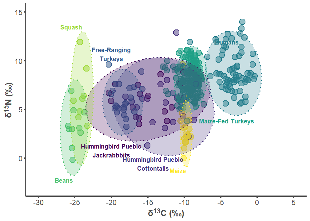
hum_p2 <- ggplot(hum_plot, aes(x = d13C, y = d15N)) +
labs(x = "δ<sup>13</sup>C (‰)",
y = "δ<sup>15</sup>N (‰)") +
theme_classic() +
theme(legend.position = "none",
axis.line = element_line(color = "#4d4d4d", linewidth = 1),
axis.text.x = element_text(color = "#4d4d4d", size = 12),
axis.text.y = element_text(color = "#4d4d4d", size = 12),
axis.title.x = element_markdown(color = "#4d4d4d", size = 14,
face = "bold"),
axis.title.y = element_markdown(color = "#4d4d4d", size = 14,
face = "bold"),
axis.ticks.x = element_line(color = "#4d4d4d", linewidth = 1),
axis.ticks.y = element_line(color = "#4d4d4d", linewidth = 1)) +
scale_color_viridis_d() +
stat_ellipse(aes(group = interaction(group), color = group, fill = group),
alpha = 0.5, linewidth = 1.1, linetype = 1, level = 0.40, type = "t",
geom = "polygon") +
stat_ellipse(aes(group = interaction(group), color = group, fill = group),
alpha = 0.25, linewidth = 0.75, linetype = 3, level = 0.95,
type = "t", geom = "polygon") +
geom_text(data = hum_label_df,aes(x = d13C, y = d15N,
label = label, color = group, hjust = hjust,
vjust = vjust),
size = 10/.pt, fontface = "bold") +
scale_fill_viridis_d() +
scale_x_continuous(limits=c(-30, 5),
breaks = c(-30, -25, -20, -15, -10, -5, 0, 5)) +
scale_y_continuous(limits=c(-3, 15))
hum_p2
10.3 Tijeras TDF
tij_label_df <- data.frame(
group = c("Tijeras Pueblo Lepus", "Tijeras Pueblo Sylvilagus",
"Free-ranging Turkey", "Humans", "Maize-fed Turkey", "Bean",
"Squash", "Corn"),
label = c("Tijeras Pueblo\nJackrabbbits",
"Tijeras Pueblo\nCottontails",
"Free-Ranging\nTurkeys", "Humans", "Maize-Fed Turkeys", "Beans",
"Squash", "Maize"),
d13C = c(-21, -17.5, -17.25, -5.8, -8, -25.25, -24, -9.75),
d15N = c(1.5, -1.75, 9.5, 12.2, 4.1, -2, 13.25, -1),
hjust = c(0.5, 0.5, 0.5, 0, 0, 1, 1, 1),
vjust = c(1, 0, 0, 1, 1, 1, 0, 1))
tij_label_df$group <- factor(tij_label_df$group,
levels = c("Tijeras Pueblo Lepus",
"Tijeras Pueblo Sylvilagus",
"Free-ranging Turkey", "Humans",
"Maize-fed Turkey", "Bean", "Squash",
"Corn"))
tij_plot <- SIBER_data_tdf %>%
filter(group %in% c("Tijeras Pueblo Lepus",
"Tijeras Pueblo Sylvilagus",
"Bean", "Corn", "Squash", "Free-ranging Turkey",
"Maize-fed Turkey", "Humans"))
tij_plot$group <- factor(tij_plot$group,
levels = c("Tijeras Pueblo Lepus",
"Tijeras Pueblo Sylvilagus",
"Free-ranging Turkey", "Humans",
"Maize-fed Turkey", "Bean", "Squash",
"Corn"))
tij_p1 <- ggplot(tij_plot, aes(x = d13C, y = d15N)) +
geom_point(aes(fill = group, color = group), stroke = 1, size = 4,
alpha = 0.5, shape = 21) +
geom_point(aes(color = group), fill = NA, stroke = 1, size = 4,
shape = 21) +
labs(x = "δ<sup>13</sup>C (‰)",
y = "δ<sup>15</sup>N (‰)") +
theme_classic() +
theme(legend.position = "none",
axis.line = element_line(color = "#4d4d4d", linewidth = 1),
axis.text.x = element_text(color = "#4d4d4d", size = 12),
axis.text.y = element_text(color = "#4d4d4d", size = 12),
axis.title.x = element_markdown(color = "#4d4d4d", size = 14,
face = "bold"),
axis.title.y = element_markdown(color = "#4d4d4d", size = 14,
face = "bold"),
axis.ticks.x = element_line(color = "#4d4d4d", linewidth = 1),
axis.ticks.y = element_line(color = "#4d4d4d", linewidth = 1)) +
scale_color_viridis_d() +
stat_ellipse(aes(group = interaction(group), color = group, fill = group),
alpha = 0.25, linewidth = 0.75, linetype = 3, level = 0.95,
type = "t", geom = "polygon") +
geom_text(data = tij_label_df,aes(x = d13C, y = d15N,
label = label, color = group, hjust = hjust,
vjust = vjust),
size = 10/.pt, fontface = "bold") +
scale_fill_viridis_d() +
scale_x_continuous(limits=c(-30, 5),
breaks = c(-30, -25, -20, -15, -10, -5, 0, 5)) +
scale_y_continuous(limits=c(-3, 15))
tij_p1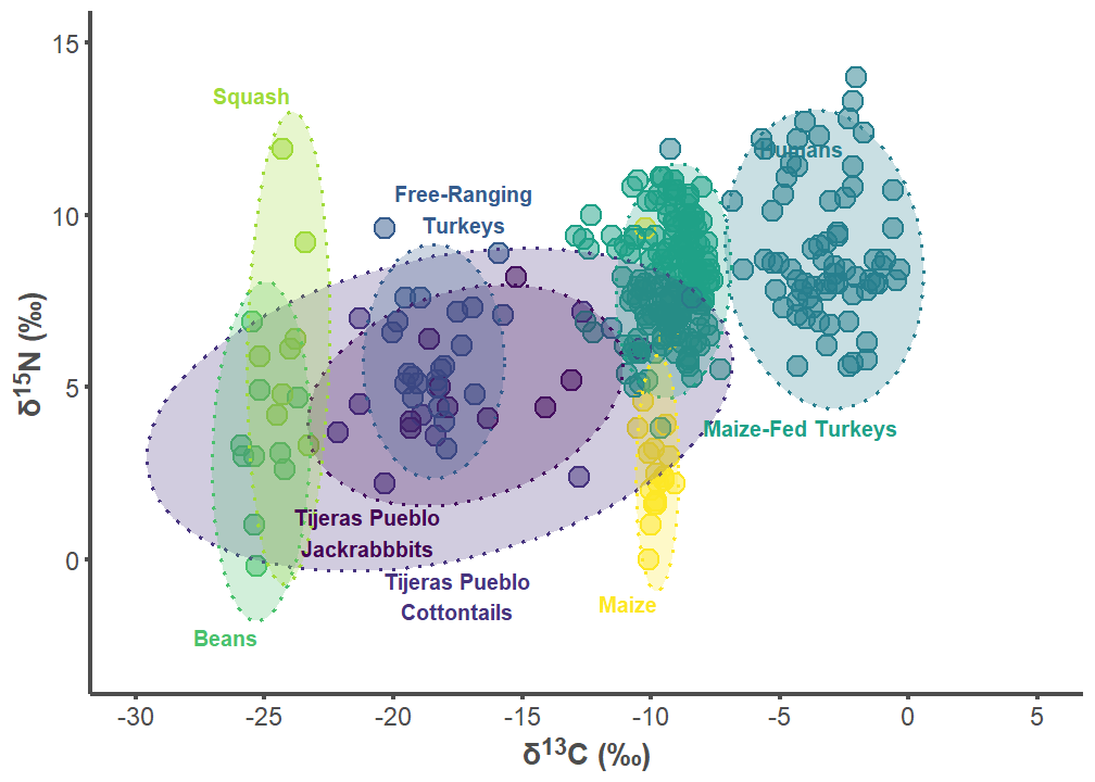
tij_p2 <- ggplot(tij_plot, aes(x = d13C, y = d15N)) +
labs(x = "δ<sup>13</sup>C (‰)",
y = "δ<sup>15</sup>N (‰)") +
theme_classic() +
theme(legend.position = "none",
axis.line = element_line(color = "#4d4d4d", linewidth = 1),
axis.text.x = element_text(color = "#4d4d4d", size = 12),
axis.text.y = element_text(color = "#4d4d4d", size = 12),
axis.title.x = element_markdown(color = "#4d4d4d", size = 14,
face = "bold"),
axis.title.y = element_markdown(color = "#4d4d4d", size = 14,
face = "bold"),
axis.ticks.x = element_line(color = "#4d4d4d", linewidth = 1),
axis.ticks.y = element_line(color = "#4d4d4d", linewidth = 1)) +
scale_color_viridis_d() +
stat_ellipse(aes(group = interaction(group), color = group, fill = group),
alpha = 0.5, linewidth = 1.1, linetype = 1, level = 0.40,
type = "t", geom = "polygon") +
stat_ellipse(aes(group = interaction(group), color = group, fill = group),
alpha = 0.25, linewidth = 0.75, linetype = 3, level = 0.95,
type = "t", geom = "polygon") +
geom_text(data = tij_label_df,aes(x = d13C, y = d15N,
label = label, color = group, hjust = hjust,
vjust = vjust),
size = 10/.pt, fontface = "bold") +
scale_fill_viridis_d() +
scale_x_continuous(limits=c(-30, 5),
breaks = c(-30, -25, -20, -15, -10, -5, 0, 5)) +
scale_y_continuous(limits=c(-3, 15))
tij_p2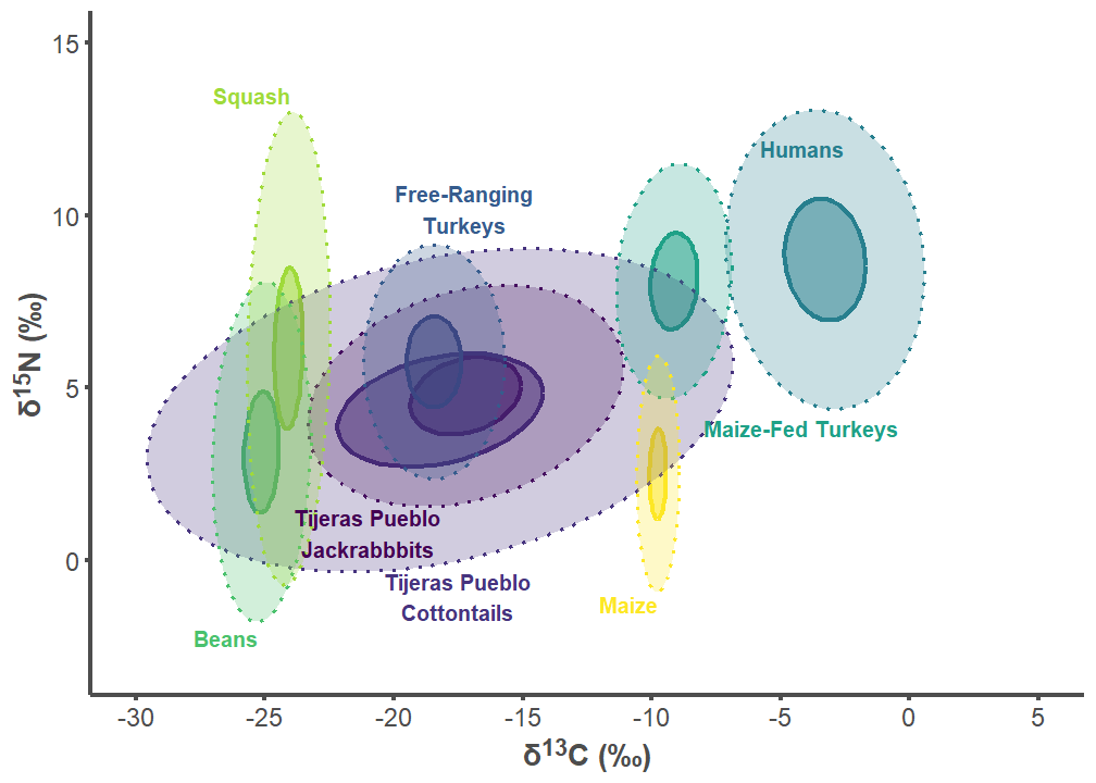
10.4 All TDF Plots
all_plots <- plot_grid(sand_p1, sand_p2, hum_p1, hum_p2, tij_p1, tij_p2,
                       labels = "AUTO", label_colour = "#4d4d4d",
                       label_size = 20, ncol = 2, nrow = 3)

all_plots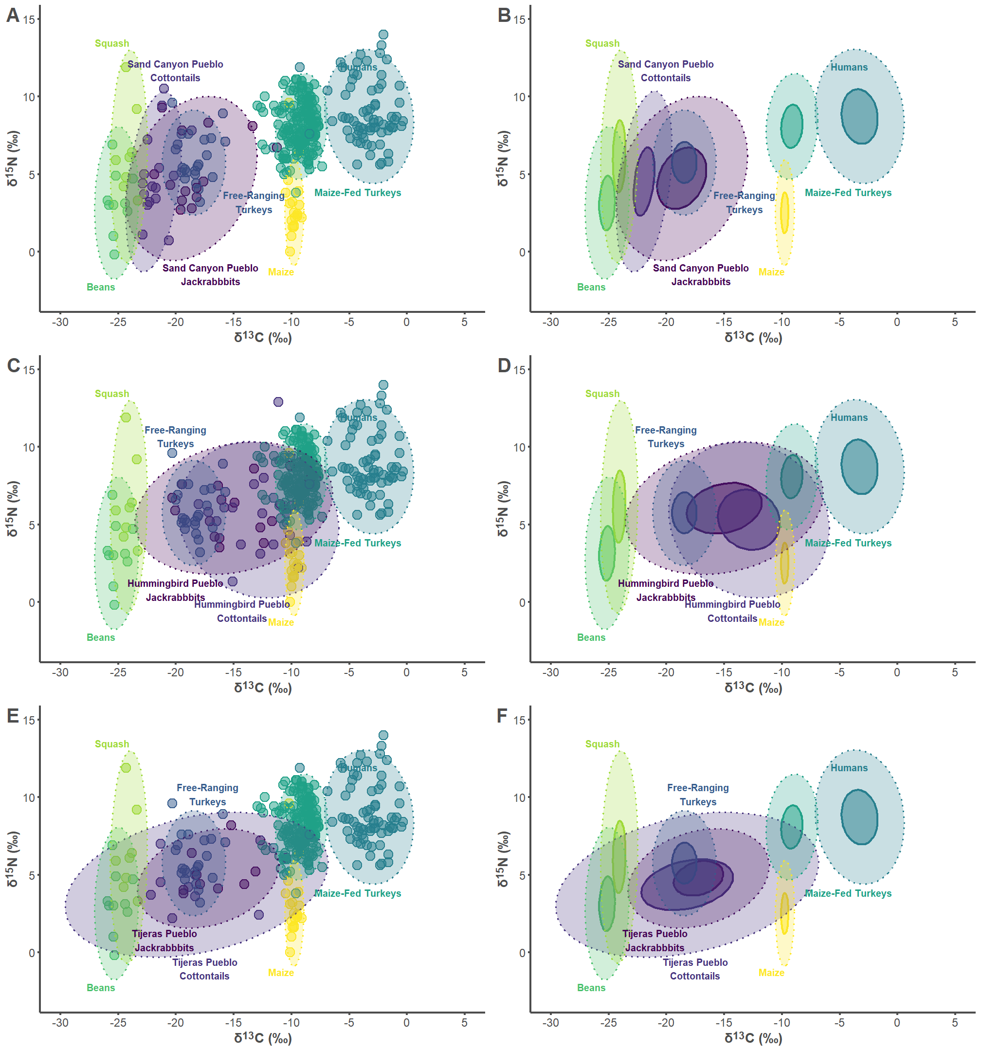
11 References
Ambrose, Stanley H. 1990. “Preparation and Characterization of Bone and Tooth Collagen for Isotopic Analysis.” Journal of Archaeological Science 17 (4): 431–51. https://doi.org/10.1016/0305-4403(90)90007-r.
Basinger, Mark A., and Phillip A. Robertson. 1997. “Vascular Flora of an Old-Growth Forest Remnant in the Ozark Hills of Southern Illinois-Updated Results.” Transactions of the Illinois State Academy of Science 90 (1-2): 1–20. https://ilacadofsci.com/wp-content/uploads/2013/08/090-01MS9611-print.pdf.
Bruhl, Jeremy J., and Karen L. Wilson. 2007. “Towards a Comprehensive Survey of C3 and C4 Photosynthetic Pathways in Cyperaceae.” Aliso: A Journal of Systematic and Floristic Botany 23 (1): 99–148. https://ilacadofsci.com/wp-content/uploads/2013/08/090-01MS9611-print.pdf.
Caut, Stéphane, Elena Angulo, and Franck Courchamp. 2009. “Variation in Discrimination Factors (Δ15N and Δ13C): The Effect of Diet Isotopic Values and Applications for Diet Reconstruction” 46 (2): 443–53. https://doi.org/10.1111/j.1365-2664.2009.01620.x.
Chisholm, Brian, and R. G. Matson. 1994. “Carbon and Nitrogen Isotopic Evidence on Basketmaker II Diet at Cedar Mesa, Utah.” KIVA 60 (2): 239–55. https://doi.org/10.1080/00231940.1994.11758268.
Coltrain, Joan Brenner, Joel C. Janetski, and Shawn W. Carlyle. 2007. “The Stable- and Radio-Isotope Chemistry of Western Basketmaker Burials: Implications for Early Puebloan Diets and Origins.” American Antiquity 72 (2): 301–21. https://doi.org/10.2307/40035815.
Conrad, Cyler, Emily Lena Jones, Seth D. Newsome, and Douglas W. Schwartz. 2016. “Bone Isotopes, Eggshell and Turkey Husbandry at Arroyo Hondo Pueblo.” Journal of Archaeological Science: Reports 10: 566–74. https://doi.org/10.1016/j.jasrep.2016.06.016.
Danneberger, Karl. 1999. “Weeds: Shedding Light on an Old Foe.” Turfgrass Trends 8 (11): 1–3. https://archive.lib.msu.edu/tic/tgtre/article/1999nov.pdf.
Dombrosky, Jonathan. 2020. “A ~1000-Year 13C Suess Correction Model for the Study of Past Ecosystems.” The Holocene 30 (3): 474–78. https://doi.org/10.1177/0959683619887416.
Giussani, Liliana M., J. Hugo Cota-Sánchez, Fernando O. Zuloaga, and Elizabeth A. Kellogg. 2001. “A Molecular Phylogeny of the Grass Subfamily Panicoideae (Poaceae) Shows Multiple Origins of C4 Photosynthesis.” American Journal of Botany 88 (11): 1993–2012. https://doi.org/10.2307/3558427.
Jackson, Andrew L., Richard Inger, Andrew C. Parnell, and Stuart Bearhop. 2011. “Comparing Isotopic Niche Widths Among and Within Communities: SIBER - Stable Isotope Bayesian Ellipses in R.” Journal of Animal Ecology 80 (3): 595–602. https://doi.org/10.1111/j.1365-2656.2011.01806.x.
Jones, Emily Lena, Cyler Conrad, Seth D. Newsome, Brian M. Kemp, and Jacqueline Marie Kocer. 2016. “Turkeys on the Fringe: Variable Husbandry in “Marginal” Areas of the Prehistoric American Southwest.” Journal of Archaeological Science: Reports 10: 575–83. https://doi.org/10.1016/j.jasrep.2016.05.051.
Kellner, Corina M., Margaret J. Schoeninger, Katherine A. Spielmann, and Katherine. Moore. 2010. “Stable Isotope Data Show Temporal Stability in Diet at Pecos Pueblo and Diet Variation Among Southwest Pueblos.” In Pecos Pueblo Revisited: The Biological and Social Context, edited by Michèle E. Morgan, 79–92. Cambridge, MA: Harvard University Press.
Kennett, Douglas J., Stephen Plog, Richard J. George, Brendan J. Culleton, Adam S. Watson, Pontus Skoglund, Nadin Rohland, et al. 2017. “Archaeogenomic Evidence Reveals Prehistoric Matrilineal Dynasty.” Nature Communications 8 (1). https://doi.org/10.1038/ncomms14115.
Kocacinar, F., and R. F. Sage. 2003. “Photosynthetic Pathway Alters Xylem Structure and Hydraulic Function in Herbaceous Plants.” Plant, Cell & Environment 26 (12): 2015–26. https://doi.org/10.1111/j.1365-2478.2003.01119.x.
Martin, Steve L. 1999. “Virgin Anasazi Diet as Demonstrated Through the Analysis of Stable Carbon and Nitrogen Isotopes.” KIVA 64 (4): 495–514. https://doi.org/10.1080/00231940.1999.11758395.
McCaffery, Harlan, Robert H. Tykot, Kathy Durand Gore, and Beau R. DeBoer. 2014. “Stable Isotope Analysis of Turkey (Meleagris gallopavo) Diet from Pueblo II and Pueblo III Sites, Middle San Juan Region, Northwest New Mexico.” American Antiquity 79 (2): 337–52. https://doi.org/10.7183/0002-7316.79.2.337.
Nelson, David M. 2012. “Carbon Isotopic Composition of Ambrosia and Artemisia Pollen: Assessment of a C3-Plant Paleophysiological Indicator.” New Phytologist 195 (4): 787–93. https://doi.org/10.1111/j.1469-8137.2012.04219.x.
Osborne, Colin P., Anna Salomaa, Thomas A. Kluyver, Vernon Visser, Elizabeth A. Kellogg, Osvaldo Morrone, Maria S. Vorontsova, W. Derek Clayton, and David A. Simpson. 2014. “A Global Database of C4 Photosynthesis in Grasses.” New Phytologist 204 (3): 441–46. https://doi.org/10.1111/nph.12942.
Rawlings, Tiffany A., and Jonathan C. Driver. 2010. “Paleodiet of Domestic Turkey, Shields Pueblo (5MT3807), Colorado: Isotopic Analysis and Its Implications for Care of a Household Domesticate.” Journal of Archaeological Science 37 (10): 2433–41. https://doi.org/10.1016/j.jas.2010.05.004.
Scribner, Kim T., and Leslie J. Krysl. 1982. “Summer Foods of the Aububons Cottontail (Sylvilagus auduboni: Leporidae) on Texas Panhandle Playa Basins.” The Southwestern Naturalist 27 (4): 460–63. https://doi.org/10.2307/3670723.
Syvertsen, J. P., G. L. Nickell, R. W. Spellenberg, and G. L. Cunningham. 1976. “Carbon Reduction Pathways and Standing Crop in Three Chihuahuan Desert Plant Communities.” The Southwestern Naturalist 21 (3): 311–20. https://doi.org/10.2307/3669716.